Section 5: Fundamentals of Speaker Recognition
5.6 Similarity Score
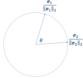
앞서 utterance/speaker가 embedding vector로 표현되는 것을 살펴보았다. 그렇다면 두 embedding vector $e_1$ , $e_2$ 가 있다고 할 때, 벡터 사이의 similarity(유사도)는 어떻게 측정할 수 있을까?
5.6.1 Cosine Similarity
대표적으로 cosine similarity를 사용하여 표현할 수 있다.
$$ \cos(e_1, e_2) = {{e_1 \cdot e_2} \over {||e_1||_2 \cdot ||e_2||_2}} $$
그림을 보며 살펴보자.
-
$e_1$ , $e_2$ 가 동일한 원점을 가진다고 가정한다.
-
$\theta$ : 두 벡터가 이루는 각도
따라서 $\cos(e_1, e_2) = \cos \theta$ 이다.
이때 만약 N-dim case일 경우, L2-normalization을 거치면서 모든 embeddings가 unit n-sphere에 위치하게 된다.
-
결과는 cosine 값이므로 [-1, 1] 사이의 값이 된다.
-
결과가 클수록 더 similar하다고 볼 수 있다.
-
extreme case
-
$\cos (e_1, e_2) = 1$ : 두 embeddings가 같은 line에 같은 방향으로 속해 있다.
-
$\cos (e_1, e_2) = 0$ : 두 embeddings가 직교한다.
-
$\cos (e_1, e_2) = 1$ : 두 embeddings가 같은 line에 있으나 서로 반대되는 방향이다.
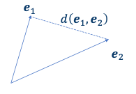
5.6.2 Euclidean Distance
다른 방법으로 Euclidean distance을 사용할 수 있다.
$$ d(e_1 , e_2) = ||e_1 - e_2 ||_2 $$
-
결과값이 벡터가 가진 length에 의해 달라진다.
-
결과가 작을수록 더 similar하다고 볼 수 있다.
따라서 역수를 취한 $d(e_1, e_2)^-1$ 을 similarity score로 사용한다.
5.6.3 Model-based similarity score
혹은 neural network를 기반으로 한 similarity score를 사용할 수 있다.
$$ f(e_1, e_2 | \theta) $$
- $f(\cdot)$ : neural network
decision network라고도 한다.
- $\theta$ : model이 가지는 parameters 집합
따라서 training dataset을 이용한 학습이 필요하다.
5.6.4 Variants
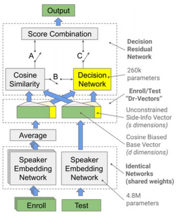
Dr-Vectors: Decision Residual Networks and an Improved Loss for Speaker Recognition 논문(2021)
이외에도 여러 방법이 있으며, 앞서 본 방법을 혼합해서 사용할 수도 있다. 예를 들어 Dr-Vectors 논문에서는 cosine similarity와 model-based score 방법을 혼합하여 similarity score를 계산한다.
이외에도 몇 가지 대표적인 variants가 있다.
- JHU variant (cosine similarity)
두 가지 trainable parameters $S$ , $b$ 를 갖는다.
Probabilistic Linear Discriminant Analysis(PLDA) 방법에서 영감을 받았다.
-
$S$ : square matrix
-
$b$ : scalar
$$ L(e_1, e_2) = {e_1}^T e_2 - {e_1}^T e_2 - {e_2}^T S e_2 + b $$
- Mahalanobis distance (Euclidean distance)
$$ d(e_1, e_2) = \sqrt{(e_1 - e_2)^T S(e_1 - e_2)} $$
5.7 Thresholding
similarity score를 계산했다면, 이제 미리 정해둔 threshold를 바탕으로 decision을 내릴 수 있다.
- Speaker Verification
score $s$ , threshold $T$
-
$s \ge T$ : same speaker
-
$s < T$ : different speaker
-
Speaker Identification
runtime embedding을 바탕으로 여러 speaker candidates에서 구분해야 한다.
따라서 multiple score를 가지며, 총 세 가지 가능성이 있다.
-
all scores < threshold: reject. imposter에 해당된다.
-
one score $\ge$ threshold: 해당 speaker로 판단한다.
-
multiple scores $\ge$ threshold: 해당 speaker 중에서 가장 높은 score를 갖는 speaker로 판단한다.
5.7.1 Multiple Threshold
하지만 decision이 꼭 Yes/No와 같은 binary일 필요는 없다. access level에 따라 여러 threshold를 두고 사용할 수도 있다.
-
low threshold
-
넘지 못할 경우: imposter로 확신(confident)한다. 모든 retry를 허락하지 않고 reject한다.
-
넘을 경우: imposter일 수 있지만 확신할 수 없다. 따라서 retry를 허락한다.
-
medium threshold
-
넘을 경우: user일 가능성이 있지만 확신할 수 없다. 따라서 limited access를 허락한다.
-
high threshold
-
넘을 경우: user로 확신한다. accept와 sensitive information 접근을 허락한다.
-
adaptative threshold
만약 score가 threshold를 넘을 경우, 현재의 utterance를 speaker profile과 함께 re-enroll한다.
5.7.2 Cosine Similarity: Threshold-friendly score
cosine similarity score는 특성상 threshold-friendly하기 때문에 가장 보편적으로 사용된다.
-
실제 계산에서 score는 [0,1] 사이 값을 갖도록 조정해서 사용한다.
-
cosine similarity: 결과값이 [-1,1]에 속한다.
-
Euclidean distance: 결과값이 [0, $\infty$ )에 속한다.
따라서 서로 다른 모델 사이의 threshold가 readable, comparable하지 않다.
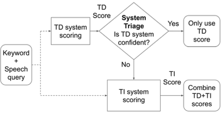
5.8 Score Triaging
경우에 따라 score를 decision을 위해 사용하지 않고, 대신 score triaging 목적으로 사용할 수 있다. 예를 들어 여러 가지 모델을 가지고 있고, 어떤 모델은 비용이 저렴한 반면 다른 모델은 비용이 크다고 하자.
다음과 같은 triage strategy를 사용한다면 훨씬 비용을 절감하면서도 성능을 유지할 수 있다.
-
Text-Dependent (small, cheap)
-
Text-Independent (big, more accurate)
-
small model(TD)이 high confidence를 갖는 경우: small model을 사용한다.
-
high confidence: cosine score가 1.0이나 0.0에 근접.
-
low confidence: cosine score가 0.5에 근접.
-
그렇지 않을 경우: TD+TI combined result를 사용한다.
5.9 Evaluation
서로 다른 system이 있을 때 evaluation이 가능하다면, 어떤 system이 더 성능이 좋은지 구분할 수 있다.
-
evaluation이 공정하기 위해서는 동일한 evaluation dataset이 필요하다.
-
단, 특정 dataset에서 system A가 B보다 성능이 좋다고 해서, 다른 dataset에서도 성능이 우수할 것이라고 보장할 수 없다.
-
training dataset이 포함한 utterances, speakers와 overlap되서는 안 된다.
또한 evaluation은 크게 Pair-based, Set-based 두 가지 방법으로 나눌 수 있다.
5.9.1 Pair-based Evaluation
Pair-based evaluation이란 trial pairs 리스트를 정의해서 evaluation을 진행하는 방식이다.
-
trial pair는 다음과 같은 요소를 포함한다.
-
two utterances
-
binary label: 두 utterances가 같은지(1), 다른지(0) 나타낸다.
예를 들어 VoxCeleb 데이터셋의 표준 trial pairs는 다음과 같은 형태이다.
• 1 id10270/x6uYqmx31kE/00001.wav id10270/8jEAjG6SegY/00008.wav
• 0 id10270/x6uYqmx31kE/00001.wav id10300/ize_eiCFEg0/00003.wav
5.9.2 Set-based Evaluation
하지만 실제 환경에서는 user가 multiple enrollment utterances를 가지고 있다. 따라서 이를 보완하기 위해 Set-based evaluation 방법을 사용한다.
- evaluation set
두 subset으로 구분하여 각 speaker마다 갖는 다른 utterances를 보완한다.
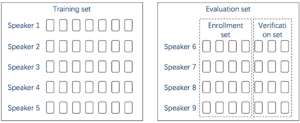
-
enrollment set
-
verification set
이러한 set-based evaluation은 두 단계로 수행된다.
-
enrollment set을 바탕으로 모든 speaker를 등록한다.
-
verification set의 utterence를 1에서 등록한 speaker와 비교한다.
-
same speaker: positive sample
-
different speaker: negative sample
그런데 verification set에서, positive samples보다 negative samples 비율이 더 많을 수밖에 없다. 따라서 subsample을 통해 positive, negative sample의 비율을 맞추는 경우가 많다.
5.10 Errors: False Accept, False Reject
utterance-vs-utterance 혹은 utterance-vs-speaker trial에 있어서 결과는 네 가지 종류로 분류할 수 있다.
| 실제 정답 | 예측 | Error |
|---|---|---|
| same speaker | same | True Accept (TA) |
| same speaker | different | False Reject (FR) = Type II Error |
| different speaker | same | False Accept (FA) = Type I Error |
| different speaker | different | True Reject (TR) |
두 종류의 오답이 발생하지 않을수록 system이 좋은 성능을 갖는다.
- False Accept Rate(FAR)
false speaker를 accept할 가능성.
$$ \mathrm{FAR} = {{\mathrm{FA}} \over {\mathrm{FA + TR}}} $$
- False Reject Rate(FRR)
true speaker를 reject할 가능성.
$$ \mathrm{FRR} = {{\mathrm{FR}} \over {\mathrm{FR + TA}}} $$
5.10.1 Errors and Threshold
이러한 errors가 발생하는 비율은 similarity score의 threshold(=operating point)에 따라서 바뀌게 된다.
-
threshold를 늘릴 경우
-
True Accept(TA) 비율이 줄어든다.
-
True Reject(TR) 비율은 늘어난다.
이처럼 threshold에 따라 FAR, FRR이 바뀌는 탓에, 다른 system을 비교할 때 그대로 FAR, FRR을 사용해서 성능을 비교할 수 없다.
5.10.2 Receiver Operation Characteristic(ROC) curve
따라서 서로 다른 system을 비교하기 위해서는 threshold-independent metrics가 필요하다. Receiver Operation Characteristic(ROC) curve는 threshold 값의 범위를 고정하여 서로 다른 system을 분석한다.(예: [0,1])
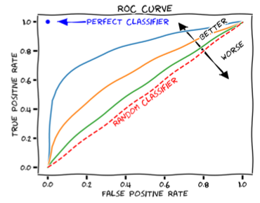
-
x축: False Accept Rate
-
y축: True Accept Rate
-
대각선에 해당되는 직선: 50:50 random guess 성능을 의미한다.
-
좌측 상단에 가까울수록 system 성능이 좋다.
ROC curve를 정량적으로 계산하기 위해 주로 사용하는 방법으로는, curve 아래 면적을 계산하는 Area Under Curve(AUC)가 있다.
-
AUC가 클수록 system 성능이 좋다.
-
[0,1] 사이 값을 갖는다.
단, AUC는 implementation과 resolution에 굉장히 sensitive하므로 주의해야 한다.
5.10.3 Detection Error Tradeoff(DET) curve
하지만 speaker recognition에서는 ROC curve보다도 Detection Error Tradeoff(DET) curve를 더 많이 사용한다.
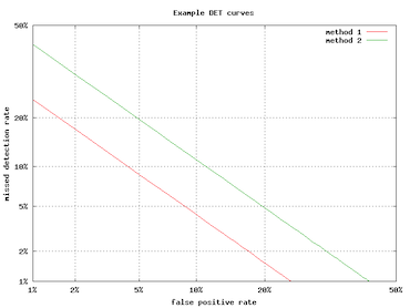
-
x축: FAR
-
y축: FRR
-
좌측 하단에 가까울수록 system 성능이 좋다.
linear하게 표시하기 위해서 대체로 log-scale을 사용한다.
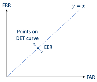
이때 DET curve에서 y=x 직선을 긋는다면, FAR=FRR이 되는 Equal Error Rate(EER) 지점이 된다.
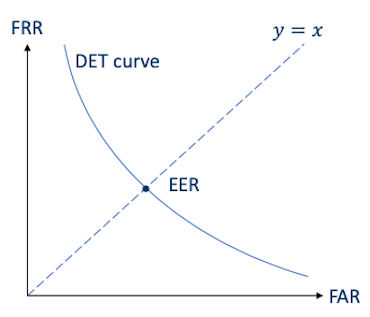
-
해당 지점에서의 threshold를 EER threshold라고 한다.
-
EER이 작을수록 system 성능이 좋다.
5.10.3.1 Computing EER
EER의 정의는 직관적이지만, 실제 계산을 통해 EER을 구하는 것은 쉽지 않다. 계산은 다음과 같은 과정으로 진행된다.
- FAR과 FRR의 값이 근접한 두 지점을 고른다.
이때 binary search 방법을 사용해서 찾는다.
- 두 지점을 이은 직선과, y=x 직선과의 교점을 찾는다.
5.10.3.2 Interpreting EER
그렇다면 이렇게 찾아낸 EER은 어떻게 해석해야 할까? 먼저 operating point를 EER threshold로 둔다고 가정하고 두 예시를 살펴보자.
- all trials = positive trials(same speaker)일 경우
"FRR $\approx$ EER, FAR = 0"이 된다.
- all trials = negative trials(different speaker)일 경우
"FAR $\approx$ EER, FRR = 0"이 된다.
EER은 충분히 total error rate의 근사값으로 사용할 수 있다. 하지만 몇몇 특수한 경우에서는 total error rate의 근사값으로 EER을 사용한다면 잘못된 비교를 저지를 수 있다.
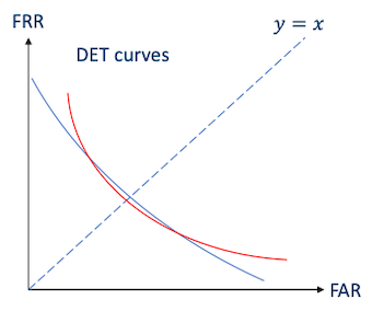
-
빨간색 DET curve의 EER < 파란색 DET curve의 EER
-
하지만 대부분의 지점에서 파란색 DET curve가 원점과 더 가깝기 때문에 성능이 더 좋다.
5.10.4 Minimun Detection Cost Function(minDCF)
또 다른 대표적인 metric으로는 Minimun Detection Cost Function(minDCF)가 있다. 특히 다른 application 간의 비교에서 많이 사용된다.
- 다른 apllications일 경우, error type마다의 tolerance level이 서로 다를 수 있다.
예를 들어 security applications에서는 FA의 위험이 크지만, wake-up application은 FR의 위험이 크다.
우선 Detection Cost Function(DCF)의 수식은, FRR, FAR별 갖는 cost를 고려하여 다음과 같이 정의된다.
$$ C_{Det} = C_{FR} \cdot \mathrm{FRR} \cdot P_T + C_{FA} \cdot FAR \cdot P_I $$
-
$C_{Det}$ : detection cost function
-
$C_{FR}$ : FR cost
-
$C_{FA}$ : FA cost
-
$P_T$ : prior probability of true speaker
-
$P_I$ : prior probability of false speaker(imposter)
여기서 minDCF는 $C_{Det}$ 가 최소값을 갖는 threshold를 찾는다.
이때 security에서는 $C_{FA}$ 를 크게 설정하고, wake-up에서는 $C_{FR}$ 을 크게 설정한다.
5.11 Identification accuracy
앞서 EER/AUC/minDCF는 speaker verification에서 사용하는 metric이었다. speaker identification에서는 주로 identification accuracy를 metric으로 사용한다.
-
utterence-vs-speaker trial pairs 대신 $(k+1)$ tuples를 사용한다.
-
evaluate할 utterance를 포함한다.
-
(true speaker 포함) $k$ different enrolled speakers를 갖는다.
-
해당 utterance를 $k$ speakers 중에서 true speaker에게 가장 높은 score를 매길수록 identification accuracy가 높다.
대체로 $k$ 를 크게 잡을수록 accuracy가 낮아진다.
5.12 Summary of metrics
다음은 metric의 dependency를 정리한 도표다. 이중에서는 EER이 다른 요인에 영향을 받지 않기 떄문에 가장 보편적으로 사용된다.
| Metrics | Depends on |
|---|---|
| FAR / FRR | threshold |
| Area under ROC curve(AUC) | Resolution of threshold / implementation details |
| Equal Error Rate(EER) | - |
| DCF | threshold, costs of FA/FR, prior probabilities of true/false speaker |
| minDCF | costs of FA/FR, prior probabilities of true/false speaker |
| Identification accuracy | number of candidate speakers $k$ |
5.13 Score Normalization
하지만 앞서 threshold를 설정할 때, 모든 speaker가 동일한 global threshold를 가지도록 했다. 그러나 이는 각 speaker의 특징을 반영하지 못하는 단점이 있다.
- 예를 들어 어떤 speaker는 더 "varied"한 목소리를 가질 수 있고, 반면 어떤 speaker는 비교적 "constant"한 목소리를 가질 수 있다.
이러한 차이가 embedding space에서의 distribution 차이를 만든다.
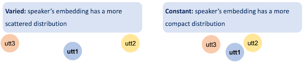
따라서 scores variabilities를 줄이기 위한 Score normalization 방법이 필요하다.
-
speaker-dependent threshold를 얻을 수 있다.
-
domain adaptation에 유리하다.
이미 domain A data으로 학습한 model에, domain B data의 샘플을 이용하여 score normalization을 수행하면, domain B data에서 더 나은 성능을 얻을 수 있다.
이러한 score normalization은 training과 evaluation 단계 사이에서 수행하는 fine-tuning 단계로 볼 수 있다. 따라서 test data를 사용해서는 안 되며(cheating) training data(혹은 hold-out dev data)를 사용해야 한다.
5.13.1 Z-norm
표준값이라고도 불리는 Z-norm(Zero normalization, Z score)을 사용할 수 있다.
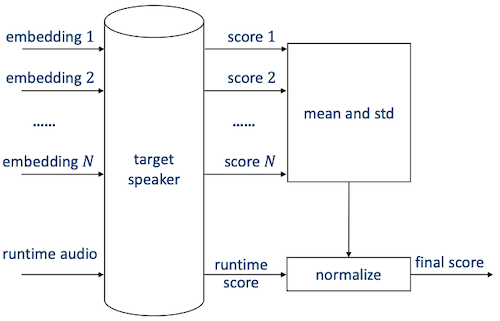
-
여러 speaker로부터 얻은 $N$ utterances를 하나의 cohort로 묶는다.
-
target speaker에 대해 $N$ uttereances의 score를 매긴다.
-
scores의 평균 $\mu$ 와 표준편차 $\sigma$ 를 구한다.
-
runtime
-
target speaker에 대한 runtime audio의 score를 매긴다.
-
score는 $\mu$ , $\sigma$ 에 의해 normalize된다.
5.13.2 T-norm
또 다른 대표적인 normalization을 방법으로는 T-norm(Test normalization)이 있다.
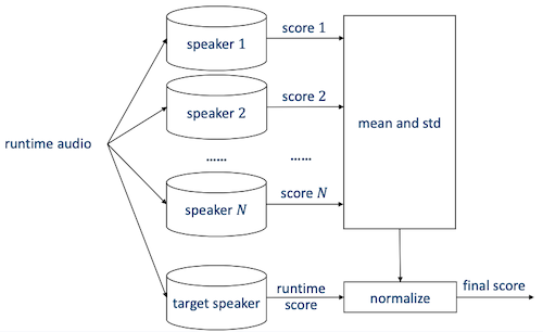
-
N speakers에 대해 runtime audio의 score를 매긴다.
-
scores의 평균 $\mu$ 와 표준편차 $\sigma$ 를 구한다.
-
target speaker에 대해 runtime audio의 score를 매긴다.
-
score는 $\mu$ , $\sigma$ 에 의해 normalize된다.
하지만 runtime에서 계산을 수행하는 만큼 computational cost가 커지고 latency가 발생한다.
5.13.3 Adaptive T-norm
Adaptive T-norm에서는 평균 $\mu$ 와 표준편차 $\sigma$ 을 구하기 위해 모든 $N$ speaker를 사용하지 않는다. 대신 target speaker와 가장 근접한 $M$ speaker subset를 사용한다. ( $M < N$ )
- 이러한 특성 덕분에 $\sigma$ 가 너무 커지는 현상도 방지할 수 있다.
5.13.4 Other normalizations
- TZ-norm
먼저 T-norm을 적용하고 Z-norm을 적용한다.
- S-norm
T-norm과 Z-norm scores를 합산한다.
Symmetric normalization의 줄임말이다.