Section 4: Acoustic Feature Extraction

Pitch detction(ACF, AMDF, Cepstrum) 정리

4.5 Two types of features

Time domain feature
- waveform samples에서 direct하게 feature를 추출한다.
- 따라서 Fourier Transform을 적용할 필요가 없다.
Frequency domain feature
- Fourier transform을 적용하여 frequency domain에서 feature를 추출한다.
- 대부분의 system이 frequency domain feature를 사용한다.

4.6 Time domain features

Time domain features는 크게 여섯 종류로 나눌 수 있다.

Short-time energy
Short-time average magnitude
Short-time zero cross rate(ZCR)
Short-time auto-correlation
Short-time average magnitude difference function (AMDF)
Short-time linear predictive coding

4.6.1 Short-time energy and average magnitude

주로 Voice Activity Detection(VAD)에서 사용된다.

Voice Activity Detection(VAD): speech signal에서 speech와 non-speech(silence) segment를 구분하는 task. 일반적으로 speech의 energy가 더 크게 나타난다.

framed sample $x [n]$ 이 있다고 하자.

$0 \leq n \leq N - 1$
$N$ : frame 내 #samples

Short-time energy $E_{x}$ 는 다음과 같이 정의할 수 있다.

E_{x} = \sum_{n = 0}^{N - 1} (x [n])^{2}

제곱항이 있는 이유는 small, large magnitude 간의 차이를 amplifiy하기 위해서이다.

Short-time average magnitude $M_{x}$ 는 다음과 같이 정의한다.

M_{x} = \frac{1}{N} \sum_{n = 0}^{N - 1} | x [n] |

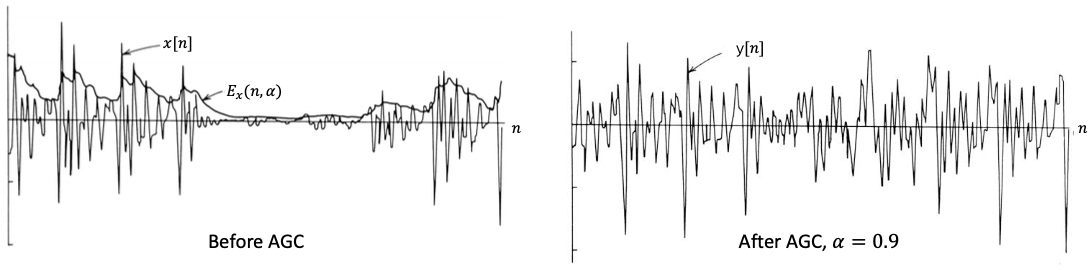
4.6.1.1 Use case: Automatic Gain Control

input magnitude가 가변적이더라도, output magnitude를 일정한 크기로 유지하고 싶을 때가 있다. 이를 위한 방법인 Automatic Gain Control(AGC)은 다음과 같이 정의한다.

E_{x} (n, α) = (1 - α) \sum_{i = - \infty}^{N - 1} α^{n - i - 1} (x [i])^{2}

= (1 - α) (x^{2} [n - 1] + α x^{2} [n - 2] + \dots)

$0 < α < 1$
After AGC: $y [n] = x [n] / \sqrt{E_{x} (n, α)}$

다음은 AGC를 적용한 후의 magnitude를 시각화한 예시이다.

AGC example

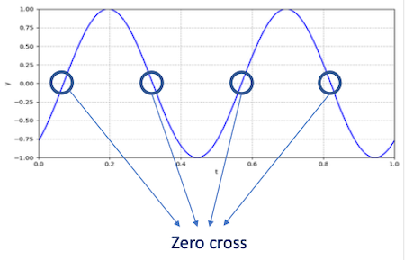
4.6.2 Short-time zero cross rate

가장 기본적인 Pitch Detection Algorithm으로 사용되었다.

Zero Cross Rate(ZCR)는 이름 그대로 얼마나 자주 $y = 0$ 을 cross하는지의 비율을 나타낸다.(= signal 부호가 바뀌는 비율)

frequency와의 correlation을 갖는다.

ZCR

수식으로 Short-time ZCR을 표현하면 다음과 같다.

Z_{x} = \frac{1}{2} \sum_{n = 1}^{N - 1} | s g n (x [n]) - s g n (x [n - 1]) |

이때 $s g n$ 함수는 다음과 같다.

s g n (x) = {\begin{matrix} 1, & i f x > 0 \\ - 1, & i f x < 0 \end{matrix}

4.6.3 Short-time autocorrelation

주로 noise를 포함한 signal에서 주기 검출을 위해 사용한다.

short-time autocorrelation은 $k$ samples만큼 delay한 signal과 original signal 사이의 correlation을 구한다. 수식은 다음과 같다.

R_{x} (k) = \sum_{n = 0}^{N - 1 - k} x [n] \cdot x [n + k]

pitch detection에서 유용하다.
$k$ 가 period의 배수일 때 correlation이 최대가 된다.

4.6.4 Short-time average magnitude difference function

Average Magnitude Difference Function(AMDF)는 $k$ samples만큼 delay한 signal과 original signal 사이의 차이를 구한다.

우선 difference는 다음과 같이 정의할 수 있다.

d_{x} (n, k) = x [n] - x [n - k]

만약 periodic signal이라면, 주기 $T$ 일 때 다음과 같이 difference는 0이 된다.

d_{x} (n, T) = 0

Short-time AMDF는 다음과 같이 정의한다.

γ_{x} (k) = \sum_{n = 0}^{N - 1 - k} | x [n + k] - x [n] |

pitch detection에서 유용하다.
- 곱셈 연산을 하는 Short-time autocorrelation과 달리, 뺄셈 연산인 만큼 연산량이 더 적다는 장점을 갖는다.
- 하지만 정확성 측면에서는 성능이 떨어진다.

4.6.5 Short-time linear predictive coding

automatic speech나 speaker recognition에서 활용한다. 예를 들어 음성 생성 모델의 parameter(특히 vocal tract filter)를 예측하는 데 사용한다.

낮은 bit rate의 신호 표현(압축)을 위해 사용할 수도 있다.

다음과 같이 각 sample을 previous sample의 linear combination으로 근사할 수 있다고 가정한다. 이 가정을 통해 과거의 samples로 현재 sample을 예측할 수 있다.

앞서 audio coding(Section03)에서 다룬 Linear Predictive Coding 식을 다시 살펴보자.

x [n] = \tilde{x} [n] + e [n] = \sum_{i = 1}^{p} a_{i} x [n - i] + e [n]

이때 $n = p, . . ., N - 1$ 에서 prediction error $e [n]$ 을 0으로 두면 연립 일차 방정식(system of linear equations)을 얻을 수 있다.

equation 수: $N - p$
LPC coefficients: $a_{1}, . . ., a_{p}$

이제 연립 방정식의 해(coefficients)를 찾아야 한다. 이는 least squares method(LSQ) 방법을 이용하여 얻을 수 있다.

solution ${a_{i}}_{1 \leq i \leq p}$

short-time features group으로써 쓰인다.
Linear Predictive Cepstral Coefficient(LPCC)
- 2번째: $1 < m < p$
- 3번째: $m > p$

C_{0} = \ln p

C_{m} = α_{m} + \sum_{k = 1}^{m - 1} \frac{k}{m} C_{k} α_{m - k}

C_{m} = \sum_{k = m - p}^{m - 1} \frac{k}{m} C_{k} α_{m - k}

4.7 Frequency domain features

frequency domain features를 얻기 위해서는, signal 종류에 따라 다양한 방식의 Fourier analysis을 적용해야 한다.

Type of signal	Fourier analysis method
Periodic continuous signal	Fourier series
Non-periodic continuous signal	Continuous Fourier transform
Periodic discrete sequence	Discrete Fourier series
Non-periodic discrete sequence	Discrete-time Fourier transform
Finite discrete sequence	Discrete Fourier transform

4.7.1 Discrete Fourier Transform

DFT 정리

Short-time analysis에서 framing, window function을 적용한 samples의 각 frame은 finite discrete sequence이다. 따라서 Discrete Fourier Transform(DFT)를 적용한다.

x [n]

를 time index $0 \leq n \leq N - 1$

에서의 sequence로 가정했을 때, DFT 수식은 다음과 같다.( $N$

: input size )

\hat{x} [k] = \sum_{n = 0}^{N - 1} \exp (- i \frac{2 π}{N} n k) \cdot x [n]

frequency index $0 \leq k \leq N - 1$
$i$ : imaginary unit(허수)

DFT는 다음과 같은 특징을 갖는다.

$\hat{x} [k]$ 는 complex number(복소수)이다.
magintude $| \hat{x} [k] |$ : $N$ features.
phase: 보통 무시한다.
계산 복잡도는 $O (N^{2})$ 이다.
- $N$ outputs $(\hat{x} [k])$
- 각 output은 $N$ 개 inputs $(x [n])$ 을 갖는다.

4.7.2 Fast Fourier Transform

DFT의 계산 복잡도를 줄이기 위해 divide-and-conquer 방식을 적용한 것이 바로 Fast Fourier Transform(FFT)이다.

계산 복잡도는 $O (N \log N)$ 이다.
input size $N$ 은 대부분의 경우에서 $2^{K}$ , 즉 2의 거듭제곱이 되도록 한다.
$N \neq 2^{K}$ 일 경우, sequence의 끝을 zero padding해야 한다. (zero padding을 통해 discontinuity 방지)

📝 예제 1: zero padding

다음 조건에서 zero padding을 적용하라.

16kHz signal, 25ms frame size
#samples per frame: 400

🔍 풀이

400 \neq 2^{K}

이다. 따라서 112 만큼 zero padding을 추가하여 $512 = 2^{9}$

가 되도록 만들고 FFT를 수행한다.

4.7.3 Short-Time Fourier Transform

Short-Time Fourier Transform(STFT)는 세 가지 step으로 구성된 개념이다.

Framing
Window function
FFT

STFT의 output을 spectrogram(스펙트로그램)으로 지칭한다.

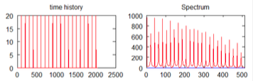
4.7.4 Cepstrum

Cepstrum을 Spectrum과의 차이를 비교하며 알아보자.

spectrum

Fourier Transform 후 output은 다음과 같은 차원을 갖는다.
- x축: frequency
- y축: magnitude
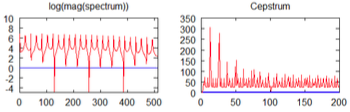
cepstrum

signal $\to$ Fourier Transform $\to$ magnitude $\to$ logarithm $\to$ inverse Fourier transform

"quefrency analysis"로도 불린다.

Spec $\to$ Ceps, freque $\to$ quefre

그렇다면 어떤 장점이 있어서 Cepstrum을 사용할까? spectrum과 비교하며 알아보자.

spectrum

time signal의 periodic structure를 분석하기 위해 사용한다.

spectrum

꽤 많은 spike가 존재한다.
cepstrum

log spectrum의 periodic structure를 분석하기 위해 사용한다.

cepstrum

특히 연산을 비교했을 때 왜 cepstrum이 유용한지 알 수 있다.

Time domain: 대부분 convolutions을 이용해서 signal을 결합한다.
Frequency domain: multiplication
Logarithm: addition

4.7.5 Demystify differency types of figures

Type of figure	x축	y축	색깔
Spectrum	Frequency	Magnitude	N/A
Phase spectrum	Frequency	Phase	N/A
Power spectrum	Frequency	Magnitude squared	N/A
Cepstrum	Quefrency	Magnitude	N/A
Spectrogram	Time	Frequency	Magnitude

4.8 Commonly used features

크게 네 가지 대표적인 feature를 살펴보자.

4.8.1 Perceptual Linear Prediction

Perceptual Linear Prediction(PLP)는 다음과 같은 절차로 진행된다.

Framing and window function

original setup: frame size fo 20ms, Hamming window
각 frame에 FFT를 적용한다.

$2^{K}$ 가 되도록 zero padding을 거친다.
power spectrum을 계산 후, Bark scale을 적용한다.
Critial-band analysis

Critical-band curve는 다음과 같이 정의된다.

Ψ (Ω) = {\begin{matrix} 0, & f o r Ω < - 1.3, \\ 10^{2.5 (Ω + 0.5)} & f o r - 1.3 \leq Ω \leq - 0.5, \\ 1 & f o r - 0.5 < Ω < 0.5, \\ 10^{- 1.0 (Ω - 0.5)} & f o r 0.5 \leq Ω \leq 2.5, \\ 0 & f o r Ω < 2.5 \end{matrix}

Equal-loudness preemphasis
Power-law for intensity

human hearing이 intensity에 nonlinear한 특성을 반영한다.

y = x^{\frac{1}{3}}

Inverse DFT

Autoregressive modeling

PLP를 발전시킨 RASTA-PLP 기법도 있다.

4.8.2 Mel-Frequency Cepstral Coefficient

Mel-Frequency Cepstral Coefficient(MFCC)는 다음과 같은 절차로 진행된다.

Preemphasis

high frequencies에서의 energy 양을 증폭시킨다.
- $0.9 \leq α < 1.0$

y [n] = x [n] - α x [n - 1]

Framming, window function
FFT on each frame
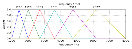
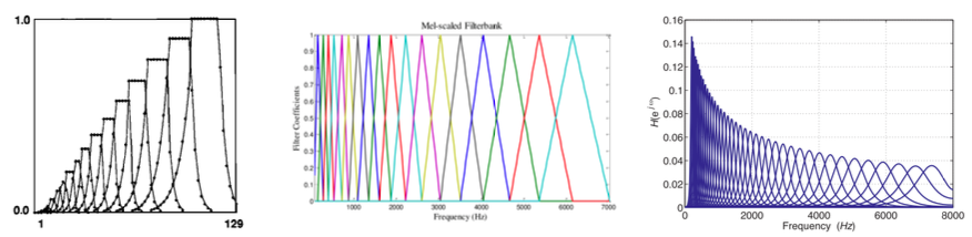
Mel filterbanks

Mel scale을 적용시킨다.(Triangular filters를 사용)
Logarithm

y = \log x

Inverse DFT

cepstrum을 계산한다.
Include deltas and energy

7번 과정의 예시를 살펴보자. inverse DFT를 거쳐 12 cepstral coefficients를 얻었다고 하자. 이제 다음과 같은 feature를 추가로 포함시킨다.

13번째 feature: energy of the frame
delta / velocity 13개: $d (t) = \frac{c (t + 1) - c (t - 1)}{2}$
double delta / acceleration 13개

최종적으로 MFCC는 $12 + 1 + 13 + 13 = 39$ 즉, 39-dimensional fiatures를 얻는다.

4.8.3 Power-Normalized Cepstral Coefficients

Power-Normalized Cepstral Coefficients(PNCC)은 PLP, MFCC와 비슷하면서 몇 가지 modification이 있는 방법이다.

Component	PLP	MFCC	PNCC
Preprocessing	N/A	Preemphasis	Preemphasis
Short-time analysis	STFT	STFT	STFT
Nonlinearity in frequency	Bark scale, critical-band	Mel-filterbanks	Gammatone filterbanks
Environmental compensation	N/A	N/A	Asymmetric noise suppression etc.
Nonlinearity in intensity	$y = x^{1 / 3}$	$y = \log x$	$y = x^{1 / 15}$
Postprocessing	Inverse DFT	Inverse DFT	Inverse DFT

위 세 가지 방법의 공통점과 차이점을 비교해 보자.

공통점
STFT를 기반으로 한다.
frequency, intensity의 nonlinearity를 compensate한다.
각 component로 어떤 방법을 사용하는가의 차이다.
차이점
사용하는 scales/filterbanks가 다르다.

각각 critical-band, Mel filterbanks, Gammatone filterbanks이다.

차이는 있으나 high frequency filter는 모두 wider하다.

4.8.4 Log-mel Filterbank Energies

Log-mel FilterBank Energies(LFBE)는 MFCC를 단순화한 방법으로 볼 수 있다. 현재 산업에서 가장 많이 사용되는 방법이다.

STFT + Mel filterbanks + Logarithm
#features: #filterbanks에 따라 결정된다.

4.9 Feature extraction in Python

다음 세 가지 Python library를 사용해서 feature를 추출할 것이다.

pip install librosa
pip install python_speech_features
pip install pyAudioAnalysis

4.9.1 MFCC in Python

다음은 librosa를 이용해서 NFCC feature extraction을 수행하는 Python 코드 예시다.

n_mfcc: n_mels보다 크면 안 된다.

deltas, energy를 포함하지 않는 구현 예제다.

S = librosa.feature.mfcc(
    y=None,             # audio waveform as time series
    sr=22050,           # y의 sampling rate
    S=None,             # spectrogram
    n_mfcc=20,          # number of MFCCs to return
    dct_type=2,         # DCT type
    norm='ortho',       # norm to use
    lifter=0,           # liftering parameter
    n_fft=2048,         # length of the FFT window(size of FFT)
    hop_length=None,    # number of samples between successive frames
    win_length=None, 
    window='hann',      # window function(Hanning)
    center=True,        # center the frames
    pad_mode='reflect', # padding method
    power=2.0           # power of the magnitude
    n_mels=128,         # number of Mel bands to generate
    fmin=0.0,           # lowest frequency
    fmax=None,          # highest frequency
)

python_speech_features를 사용한 코드는 다음과 같다.

numcep: nfilt보다 크면 안 된다.

deltas를 포함하지 않는 구현 예제다.

S = python_speech_features.base.mfcc(
    signal,              # audio waveform at time signal
    samplerate=16000,    
    winlen=0.025,        # STFT frame size at seconds
    winstep=0.01,        # STFT frame step at seconds
    numcep=13,           # number of cepstrum to return
    nfilt=26,            # number of filters
    nfft=512,            # size of FFT
    lowfreq=0,           # lowest frequency[Hz]
    highfreq=None,       # highest frequency[Hz]
    preemph=0.97,
    ceplifter=22,
    appendEnergy=True,
    winfunc=np.hanning    #
)

아래는 두 library의 argument를 비교한 도표다.

arg	librosa	python_speech_features
Input audio waveform	y	signal
Sampling rate	sr	samplerate
Output feature dimension	n_mfcc	numcep
STFT frame size	win_length	winlen
STFT frame step	hop_length	winstep
STFT window function	window	winfunc
Size of FFT	n_fft	nfft
Number of Mel bands	n_mels	nfilt
Lowest frequency	f_min	lowfreq
Highest frequency	f_max	highfreq