15 Long-Context LLM

EfficientML.ai Lecture 15 - Long-Context LLM (MIT 6.5940, Fall 2024, Zoom Recording)

긴 문서나 동영상 프레임을 이해하고 싶다고 하자. 하나의 224x224 크기 이미지를 256 token로 계산하면, 1시간 동영상 기준으로는 약 백만 개 토큰이라는 long context를 처리해야 한다.

video example

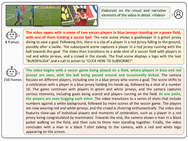
컨텍스트 길이에 따라 메모리 사용량 및 지연시간이 극적으로 증가하므로, 이를 효율적으로 처리하는 것이 중요하다. 이때 일반적인 KV cache compression 기법으로는 LLM의 long context 성능을 저하시킬 수 있으므로, 보다 효율적인 접근법이 필요하다.

백만 개 토큰 처리 기준, 137GB KV cache 메모리(Llama-3-8B), 92 ms/token 지연시간(Llama-3-7B) 발생

15.5 DuoAttention: Retrieval and Streaming Heads

DuoAttention: Efficient Long-Context LLM Inference with Retrieval and Streaming Heads 논문(2024)

DuoAttention은 long context 성능을 보존하면서 메모리 병목과 지연시간을 최적화하기 위해, 역할을 분할한 attention head 설계를 제안하였다.

Retrieval Heads: earlier context에서 중요 토큰 포착 (w. full KV cache)
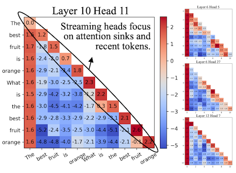
Streaming Heads: 최근 토큰 및 attention sink 집중 (w. 최근 토큰으로 구성된 reduced KV cache)

Heads	Caches

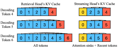노란색 토큰: attention sink, $α$ : gate value

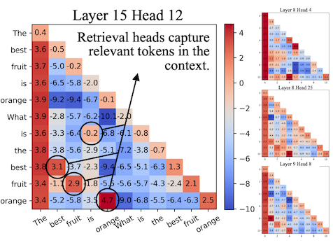
다음은 두 head의 attention map 예시로, 각 head가 어디에 집중하는지 관찰할 수 있다.

Retrieval Head	Streaming Head

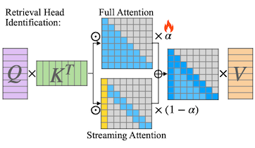
15.5.1 Identification of Retrieval Heads

DuoAttention은 LLM 가중치는 고정한 채, head를 구분하는 gate 파라미터 $α$ 만을 학습한다. ( $α$ 가 0에 가까울수록 streaming head 사용 )

gate 값에 따라 두 head의 비중 조절
full attention: $M_{c a s u a l}$
streaming attention: $M_{s t r e a m i n g}$

a t t n_{i, j} = α_{i, j} \cdot f u l l a t t n + (1 - α_{i, j}) \cdot s t r e a m i n g a t t n

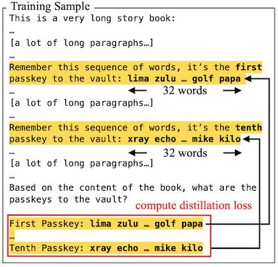
학습은 long-context passkey retrieval task로 이루어지며, passkey 추론 결과를 바탕으로 증류 손실을 계산한다.

손실 함수: full attention만 사용하는 모델에서의 증류 항 + $α$ 를 작은 값으로 유도하는 L1 정규화 항

L_{d i s t i l l} = \frac{1}{N} \sum_{i = 1}^{N} \sum_{j = T - l + 1}^{T} (H_{f u l l}^{(i)} [j] - H_{m i x e d}^{(i)} [j])^{2}, L_{r e g} = \sum_{i = 1}^{L} \sum_{j = 1}^{H} | a_{i, j} |

ℒ = L_{d i s t i l l} + λ L_{r e g}

Training Sample	Optimized Gate Value (red:1, blue:0)

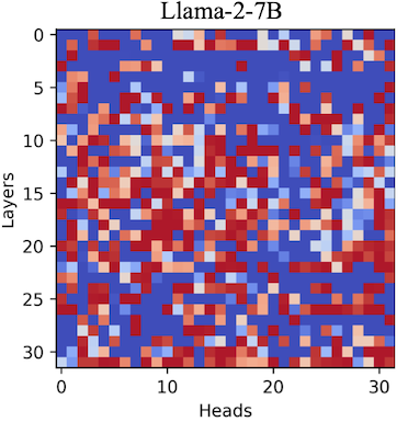e.g., Llama2-7B: 약 1천 개 $α$ 만 학습 (32개 레이어 x 32개 MHA) $\to$ 8 A100 GPUs 기준 몇 시간 내 학습

15.5.2 DuoAttention: Deployment

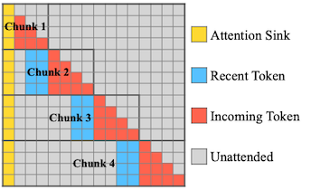
streaming head는 고정된 크기(constant)의 KV cache만을 사용하므로, chunked pre-filling에서 메모리 사용량 및 지연시간을 크게 줄일 수 있다.

Decoding	Chunked Pre-Filling

시간 복잡도: $O (L^{2}) \to O (L K)$
메모리 복잡도: $O (L) \to O (K)$

$L$ : sequence length, $K$ : chunk size

15.5.3 DuoAttention: Results

(생략)

15.6 Quest: Query-Aware Sparsity

Quest: Query-Aware Sparsity for Efficient Long-Context LLM Inference 논문(2024)

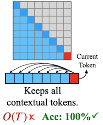
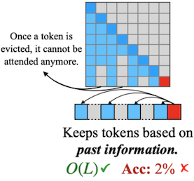
KV cache 크기를 압축하는 기존 방법은, (지금은 중요하지 않지만) 나중에 중요한 역할을 하는 token을 제거하여 복구할 수 없는 정보 손실을 유발할 수 있었다.

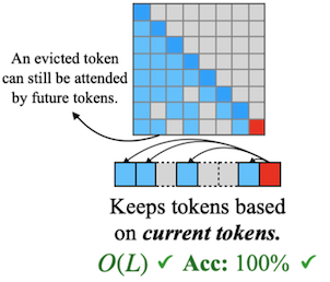
Dense Attention	Query-Agnostic Sparsity (StreamingLLM, H2O, etc.)	Query-Aware Sparsity (Quest)

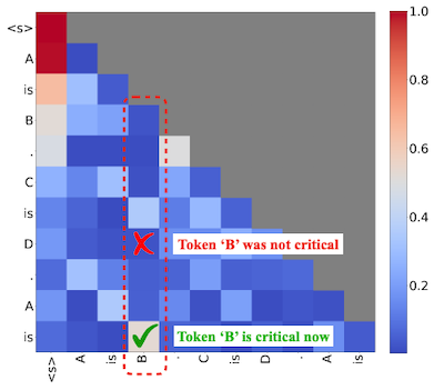
Notes: 예를 들어, 토큰 ‘B'는 (A is B 정답인 만큼) current query 'is'(마지막 'is')에서 중요하다. 그러나 이전까지는 어떠한 다른 쿼리에서도 중요하게 계산되지 않는다.

관찰: 중요도(criticality) 판단은 query vector $Q$ 에 굉장히 dependent하게 이루어진다.

15.6.1 Query-Aware Sparsity

Quest는 앞선 관찰을 토대로 KV cache page 중요도를 동적으로 계산하는 방법을 제안하였다.

Key 페이지에서 채널별 max, min 값( $M_{i}$ , $m_{i}$ )만을 메타데이터화 (Reduced Keys)

for i = 1 to dim do
   M_i = max(M_i, k_i)
   m_i = min(m_i, k_i)
end for

Current query $q$ 와 $M_{i}$ , $m_{i}$ 으로 채널별 upper bound 계산

attention weight의 upper bound를 중요도로 사용한다.

Initialize score = 0
for i = 1 to dim do
  score += MAX(q_i * max, q_i * min)
end for

중요도 점수에 따라 Top-k page만 선택하여 sparse attention 수행

quest self-attention

파란색, 주황색: 각각 K page, V page

예시의 page dim=4이나, 실제로는 16이나 64 차원을 갖는다.

15.6.2 Quest: Results

(생략)

15.7 Beyond Transformers: Mamba

Mamba: Linear-Time Sequence Modeling with Selective State Spaces 논문(2023)

Maarten Grootendorst: A Visual Guide to Mamba and State Space Models

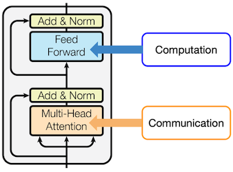
다음과 같은 관점으로 LLM의 두 가지 중요한 연산을 해석할 수 있다.

token 간 communication = Attention $\to$ Mamba's SSM
단일 token 내 computation = MLPs

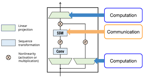
Mamba는 attention 기반의 communication을 Selective State Space Models(SSMs) 구조로 대체한다.

long sequences 대상으로 linear time processing 달성

Transformer Block	Mamba Block

15.7.1 Background: State-Space Models (SSMs)

SSM은 hidden state(입력 시퀀스에 대한 current knowledge), 입력 정보 $x_{t}$ , 출력 $y_{t}$ 간의 관계를 모델링한다.

SSM recurrent

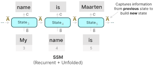
h_{t} = \bar{A} h_{t - 1} + \bar{B} x_{t}

y_{t} = C h_{t}

Matrix	Role	Description
$A$	state transition을 제어	How should I forget or update the state over time?
$B$	입력을 hidden state로 매핑	What part of the new input should I remember?
$C$	state를 출력으로 매핑	How can I use the state for a good prediction?

학습의 최적화는 Linear Recurrence가 Global Convolution와 수학적으로 동등하다는 사실을 이용한다.

\bar{K} = (C \bar{B}, C \bar{A} \bar{B}, \dots, C {\bar{A}}^{k} \bar{B}, \dots)

Step 0: $\bar{B} x_{0}$

Step 1: $\bar{A} h_{0} + \bar{B} x_{1} = \bar{A} \bar{B} x_{0} + \bar{B} x_{1}$

Step 2: $\bar{A} h_{1} + \bar{B} x_{2} = \bar{A} (\bar{A} \bar{B} x_{0} + \bar{B} x_{1}) + \bar{B} x_{2} = {\bar{A}}^{2} \bar{B} x_{0} + \bar{A} \bar{B} x_{1} + \bar{B} x_{2}$

15.7.2 Selective State-Space Model

그러나, SSM에서 행렬 $A, B, C$ 는 모든 입력에 동일(static)하므로, 불필요한 부분을 제외하고 선택적으로 집중하는 능력이 떨어진다.

Mamba는 이러한 SSM 모델의 한계를 극복하기 위해 selective mechanism을 결합하였다.

$△_{t}$ : 현재 입력 $x_{t}$ 에 집중할지 무시할지 결정 (step size)
SSM 파라미터 $(△, B, C)$ : input dependent (time-varying)

structured SSM

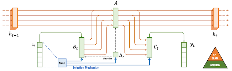
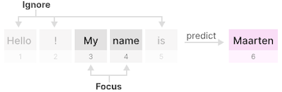
$△_{t}$ : 아래 RNN gating과 유사하게 동작하며, $x_{t}$ 에 대한 linear projection으로 계산되므로 input dependent하다.

$△_{t}$ 가 클수록 현재 입력 $x_{t}$ 에 집중 (이전 상태를 잊어버림)

$h_{t} = (1 - g_{t}) h_{t - 1} + g_{t} x_{t}$

다음 예시는 step size에 따라 focus가 변화한 모습을 보여준다.

mamba step size example

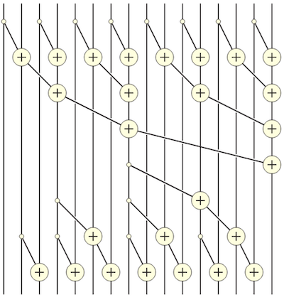
15.7.3 Fast Training using Parallel Scan

time-varying한 설계 방식의 문제는, 기존처럼 global convolution의 가속화 기법을 적용할 수 없게 만든다. 논문에서는 이를 Parallel Scan Algorithm을 활용하여 해결한다.

Notes: 배열의 'prefix sum' 계산하는 알고리즘과 유사

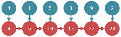
다음 예시는 hidden state $h_{0}, h_{1}, h_{2}, h_{3}$ 를 병렬로 계산하는 과정으로 이해할 수 있다.

parallel scan

15.7.4 Hybrid Models: Jamba

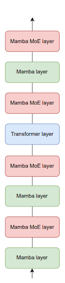
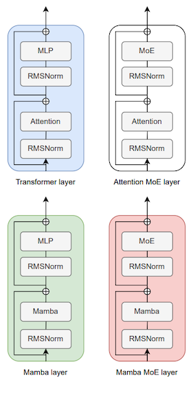
Jamba: A Hybrid Transformer-Mamba Language Model 논문(2024)

Jamba는 Mixture of Experts(MoE) 모듈을 포함해, Mamba와 Transformer 블록을 결합한 하이브리드 모델이다.

단일 Jamba Block	Different Types of Layers