13 LLM Deployment Techniques

EfficientML.ai Lecture 13 - LLM Deployment Techniques (MIT 6.5940, Fall 2024)

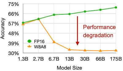
CNN과 다르게, LLM에서는 W8A8 양자화가 잘 동작하지 않는다.

• 작은 모델에서는 효과가 있지만, 모델 크기가 6.7B 이상이라면 양자화에 따른 정확도 하락이 크게 발생한다.

13.1 SmoothQuant: Weight-Activation Quantization

SmoothQuant: Accurate and Efficient Post-Training Quantization for Large Language Models 논문(2022)

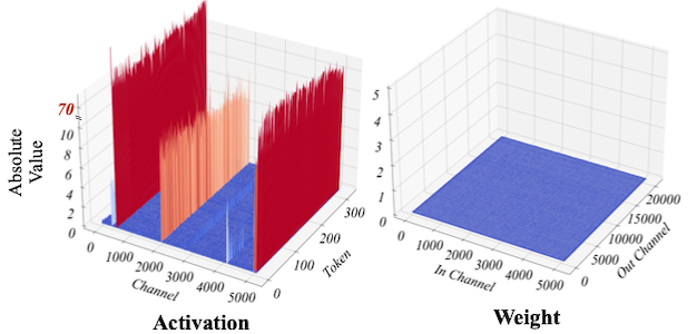
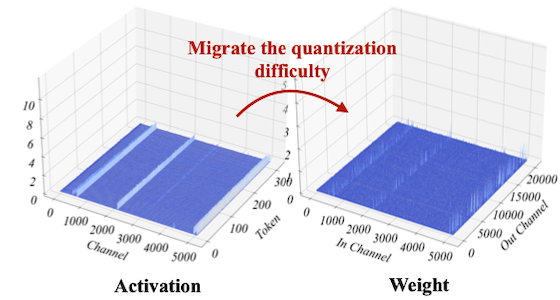
이처럼 양자화의 정확도 하락은, 주로 특정 채널의 activation 값이 다른 채널에 비해 상대적으로 큰 outlier에 의해 발생한다. 다음은 LLM의 양자화 이전 activation, weight 절댓값 분포를 채널별로 나타낸 그림이다.

• activation: outlier channel로 인해 양자화가 어렵다.

• weight: 상대적으로 균일하여 양자화가 쉽다.

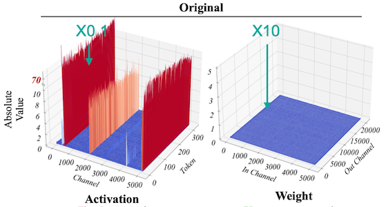
SmoothQuant에서는 activation과 weight의 행렬 곱셈(linear)에서 scaling 트릭을 적용하여 문제를 개선한다.

예를 들어 activation에 0.1을 곱한 뒤 weight에 10을 곱하면, 수학적으로 이전과 동일한 결과를 획득할 수 있다.

Difficulty	Scaling	Smoothed
Activation	Hard	Easy
Weight	Easy	Harder but still Easy

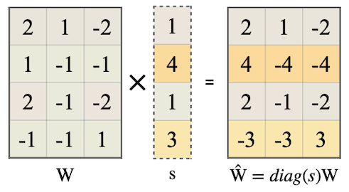
13.1.1 Activation Smoothing

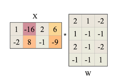
다음은 SmoothQuant에서 scaling 트릭을 적용하는 과정을 나타낸 그림이다. (왼쪽 행렬은 activation $\mathbf{X}$ , 오른쪽 행렬은 weight $\mathbf{W}$ , $\alpha$ 는 Migration Strength(논문: 0.5))

예제 activation: 2개의 sequence, 각 sequence는 4 hidden dimension(input channel $j = 1, 2, 3, 4$ )을 갖는다.

색상 하이라이트는 outlier value를 나타낸다.

(1) Calibration Stage (Offline)

per-channel smoothing factor $s$ 를 획득한다.

Per-channel Abs Max	$\max |\mathbf{X}|$ ÷ $\max |\mathbf{W}|$

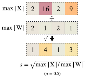$$ s_j = \max (|\mathbf{X_j}|)^{\alpha} / \max (|\mathbf{W_j}|)^{1- \alpha} $$

(2) Smoothing Stage (Offline)

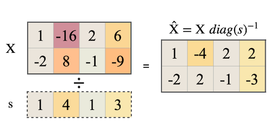
activation의 smoothing은, LayerNorm에서 $s$ 를 나누는 방식으로 통합하여 구현된다. (fuzed $\rightarrow$ zero overhead)

Activation	Weight

(3) Inference (Runtime)

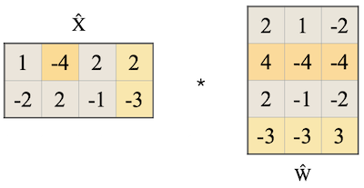
$$ \mathbf{Y} = (\mathbf{X} diag (s)^{-1}) \cdot (diag (s)\mathbf{W}) = \hat{\mathbf{X} }\hat{\mathbf{W} } $$

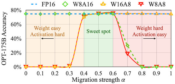
13.1.2 Ablation Study on the Migration Strength

OPT-175B 모델을 대상으로 migration strength를 다양하게 조정한 실험에서는, $\alpha$ 를 0.5에 근접하게 설정했을 때 가장 높은 정확도를 획득했다.

• $\alpha < 0.4$ : activation 난이도 상승

• $\alpha > 0.6$ : weight 난이도 상승

13.1.3 System Implementation

SmoothQuant는 (NVIDIA에서 Transformer 추론 가속을 위해 설계한) FasterTransformer 라이브러리에 기반한 시스템을 설계하였다.

• compute-intensive operations (Linear, BMM): INT8로 양자화하여 연산한다.

• LayerNorm, Softmax, Element-wise Add: 정확도를 위해 FP16으로 연산한다.

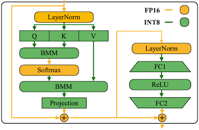
BMM: Batch Matrix Multiplication

13.1.4 SmoothQuant Benchmark

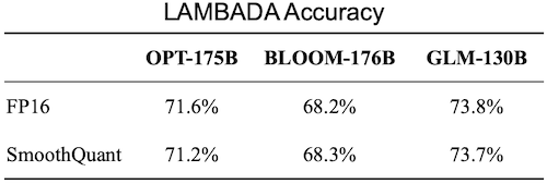
다음은 세 가지 LLM 모델을 대상으로 한 SmoothQuant 적용 전, 후 LAMBADA 벤치마크 정확도를 비교한 결과이다. (참고로 SmoothQuant는 별도의 미세조정을 필요로 하지 않는다.)

다음은 OPT-175B 모델을 대상으로 한 실험에서 SmoothQuant의 지연시간, 메모리 사용량을 비교한 도표이다.

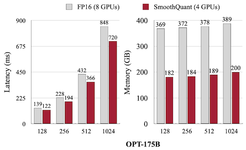
SmoothQuant를 사용하면, MT-NLG 530B 모델을 8 GPU(NVIDIA A6000)를 장착한 1개 노드만으로 서빙할 수 있다. (통신 오버헤드 제거)

13.2 Single-batch LLM Serving

앞서 SmoothQuant의 W8A8 양자화는 batch serving (e.g., bs=128)에서 효율적일 수 있으나, On-device처럼 single-query LLM inference를 가정한 시나리오에서는 대안으로 적합하지 않다.

13.2.1 Highly Memory-bounded Decoding

다음은 LLaMA-65B decoding을 수행했을 때, batch size 설정별 compute intensity를 나타낸 그림이다. (NVIDIA A100 GPU 기준)

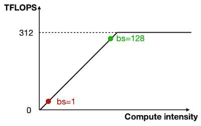
• bs=1: memory bound 병목으로, 충분한 성능을 이끌어내지 않는다.

Compute Intensity = FLOPs / Memory Bandwidth

13.2.2 Bottleneck of Single-batch LLM Inference

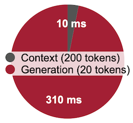
다음은 LLaMA-7B의 RTX 4090 GPU 추론(bs=1, FP16 with FasterTransformer)을 가정했을 때, context stage와 generation stage의 latency 및 computation intensity를 비교한 실험이다.

Context(summarizing a prompt with 200 tokens) vs. Generation(generating 20 tokens)

Latency	Computation Intensity(Generation Stage)

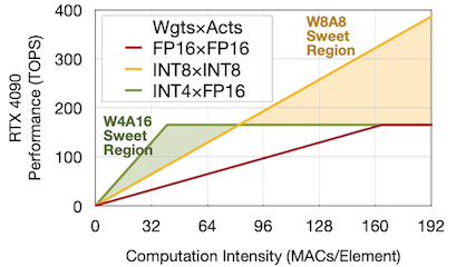이처럼 배치 사이즈가 작은 경우, 추론 지연시간의 대부분을 generation stage이 차지하는 것을 확인할 수 있다. 또한, 작은 배치 사이즈 설정에서는, W8A8보다 W4A16 양자화가 우수한 computation intensity를 가졌다.

다음은 Attention, FFN 연산에서 weight, activation의 memory footprint를 비교한 그림이다.

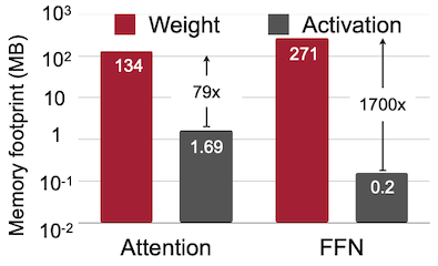
이처럼 single-batch 설정에서는 weight loading이 메모리 병목의 큰 지분을 차지한다. 하지만 달리 말하면, 가중치를 low-bit로 양자화하는 것으로 token generation을 가속할 수 있다.

13.3 AWQ: Activation-aware Weight Quantization

AWQ: Activation-aware Weight Quantization for LLM Compression and Acceleration 논문(2023)

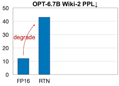
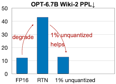
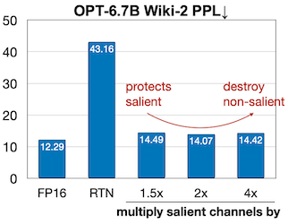
그러나, 단순한 low-bit weight quantization만으로는 LLM의 급격한 정확도 하락을 방지하기 어렵다. 다음은 OPT-6.7B 모델을 INT3 양자화했을 때 발생하는 정확도 하락을 보여준다.

Group-wise(or block-wise) quantization을 적용하였다. (group size=128)

Conventional int3-g128	Acc. Degrade

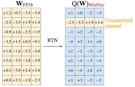
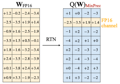
하지만 AWQ는 양자화에서 가장 중요한(salient) 1%의 가중치 채널만 예외로 두는 것으로, 발생하는 정확도 하락을 대부분 방지할 수 있다는 사실을 발견하였다.

AWQ(Mixed Precision)	Acc. Degrade

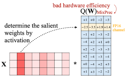
13.3.1 Selecting Salient Weight Channels

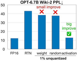
이때 1%의 중요한 가중치 채널은, activation outlier를 기준으로 선택한다.

Selected by Activation	Acc. Degrade

13.3.2 Protect Salient Weight by Scaling

하지만, FP16 mixed precision을 유지하는 것은 구현이 어렵고 비효율적이다.

Notes: 양자화는 일반적으로 다음과 같은 수식으로 정의된다. ( $y = Q(\mathbf{w})\mathbf{x}$ )

$$ Q(\mathbf{w}) = \triangle \cdot \mathrm{round} \frac{\mathbf{w} }{\triangle} $$

$$ \triangle = \frac{\max (|\mathbf{w}|)}{2^{N-1} } $$

$N$ : number of bits, $\mathbf{w}$ : group/block of weight (그룹마다 Absmax를 적용한다.)

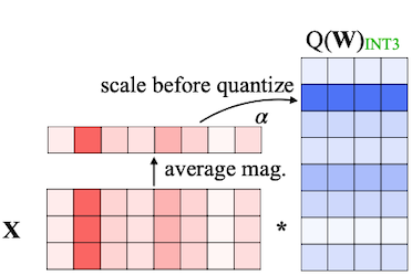
따라서 AWQ는 mixed precision을 유지하는 대신, 양자화에 scaling을 추가하여 salient weight를 보호하는 방법을 제안하였다.

$$ \mathbf{WX} \overset{Quant}{\longrightarrow} Q(\mathbf{W} \cdot \mathbf{s}) (\mathbf{s^{-1} } \cdot \mathbf{X}) $$

$\mathbf{s^{-1} }$ : 이전 연산에 결합(fused)하여 수행된다.

그러나 해당 scaling으로 발생하는 양자화 오차를 고려해야 하므로, 이를 위한 적절한 기준도 필요하게 되었다.

Scaling	Acc. Degrade

13.3.3 Activation-aware Optimal Scaling

Notes: $\mathbf{s}$ 가 너무 크지 않다는 가정( $\triangle \approx \triangle '$ ) 하에, 양자화 오차는 $\mathbf{s^{-1} }$ 에 비례한다.

• 99% weight channel

$$ Q(w) \cdot x = \triangle \cdot \mathrm{round} \frac{w}{\triangle} \cdot x $$

• 1% salient weight channel

$$ Q(w \cdot s) \cdot \frac{x}{s} = \triangle ' \cdot \mathrm{round} \frac{w \cdot s}{\triangle '} \cdot x \cdot \frac{1}{s} $$

AWQ는 양자화 전,후 activation의 차이를 최소화하는 방식으로 최적 scaling 설정을 탐색한다.

$$ \mathscr{L}(\mathbf{s}) = || Q(\mathbf{W} \cdot \mathbf{s}) (\mathbf{s^{-1} } \cdot \mathbf{X}) - \mathbf{WX} || $$

이때 $\mathbf{s}$ 의 search space는, salient channel과 non-salient channel의 균형을 맞추기 위한 하이퍼파라미터인 $\alpha \in [0, 1]$ 를 포함한다. (0: scaling 미적용) $\alpha$ 의 탐색은 grid search를 통해 진행된다.

$$ \mathbf{s} = \mathbf{s^{\alpha}_{X} } $$

$$ {\alpha}^{*} = \arg\min_{\alpha} \mathscr{L}( \mathbf{s^{\alpha}_{X} } ) $$

$\mathbf{s_{X} }$ : average magnitude of activation (per-channel)

13.3.4 Data-efficiency for Calibration Set

AWQ는 설계상 regression이나 backpropagation이 필요하지 않으며, 적은 양의 calibration set만으로도 양자화를 수행할 수 있다.

다음 도표는 AWQ와 GPTQ를 비교한 실험으로, 실제로 AWQ가 GPTQ 대비 10배 작은 calibration set에서 보다 우수한 perplexity를 갖는 것을 관찰할 수 있다.

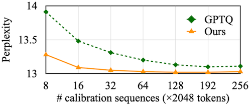
참고로 AWQ는 GPTQ와 orthogonal하기 때문에, 둘을 함께 사용하는 선택도 가능하다.

13.3.5 AWQ Results

VILA: On Pre-training for Visual Language Models 논문(2023)

다음은 Llama-2, LLaMA 모델을 대상으로 AWQ의 perplexity를 비교한 실험 결과이다. (INT3-g128, INT4-g128)

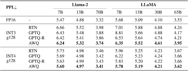
RTN: Round-to-nearest quantization

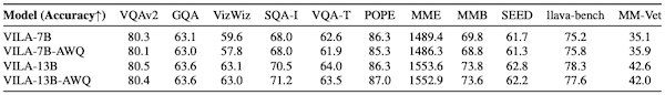
또한, VLM(Vision Language Model)인 VILA 모델을 대상으로 한 실험에서도 우수한 성능을 달성하였다.