12 Transformer and LLM (Part I)
EfficientML.ai Lecture 12 - Transformer and LLM (Part I) (MIT 6.5940, Fall 2023, Zoom)
Transformer의 등장 이후, 이를 기반으로 한 다양한 설계가 제안되었다.
-
Encoder-Decoder(T5), Encoder-only(BERT), Decoder-only(GPT)
-
Absolute Positional Encoding $\rightarrow$ Relative Positional Encoding
-
KV cache optimizations
Multi-Head Attention(MHA) $\rightarrow$ Multi-Query Attention(MQA) $\rightarrow$ Grouped-Query Attention(GQA)
- FFN $\rightarrow$ GLU(Gated Linear Unit)
12.4 Types of Transformer-based Models
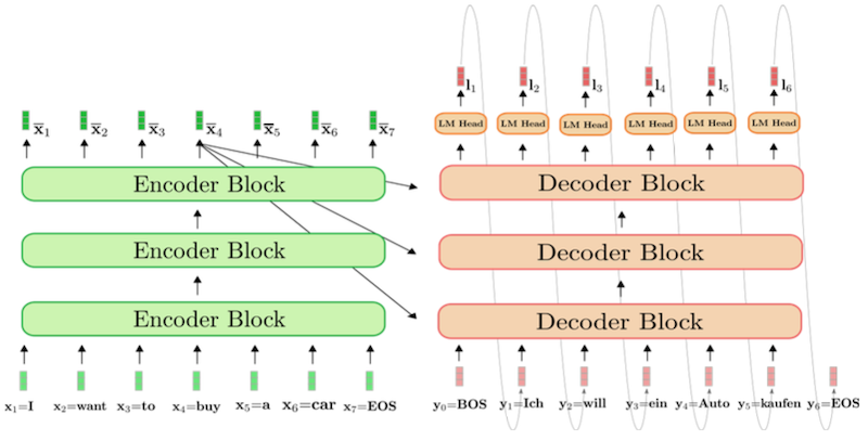
original Transformer는 Encoder-Decoder 구조를 가지고 있다.
12.4.1 Encoder-Decoder: T5
Exploring the Limits of Transfer Learning with a Unified Text-to-Text Transformer 논문(2019)
위 논문에서는 다양한 NLP task를 text-to-text 포맷(텍스트 입력-텍스트 출력)으로 통일한 프레임워크를 제안했다.
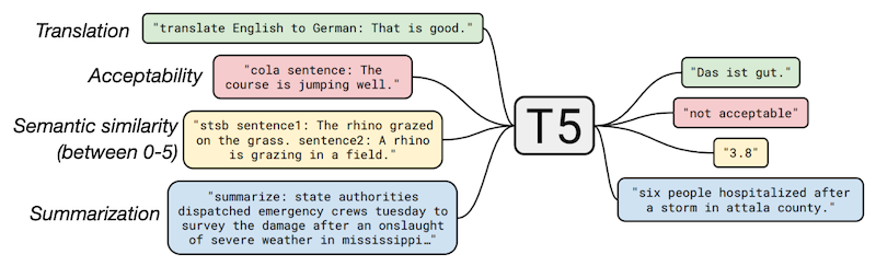
해당 논문의 T5 모델은 대표적인 Encoder-Decoder 아키텍처로, 다양한 NLP task에서 전이 학습에 기반해 최첨단 성능을 획득하였다.
- encoder에 prompt를 제공하면, decoder에서 answer 텍스트을 생성한다.
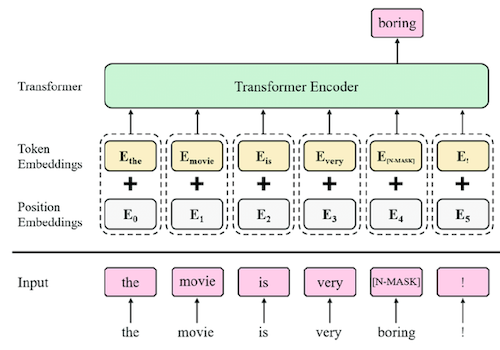
12.4.2 Encoder-only: BERT
BERT: Pre-training of Deep Bidirectional Transformers for Language Understanding 논문(2018)
대표적인 Encoder-only 모델인 BERT는, 대규모 비지도 사전학습 단계에서 2개의 objective를 동시에 가진다.
| Objective | Description |
|---|---|
| Masked Language Model(MLM) | 입력 token에서 임의로 선택된 단어를 마스킹(15%)하고, 마스킹된 단어를 예측하는 task |
| Next Sentence Prediction(NSP) | 두 문장 A, B가 주어졌을 때, B가 A의 다음 문장인지 예측하는 task |
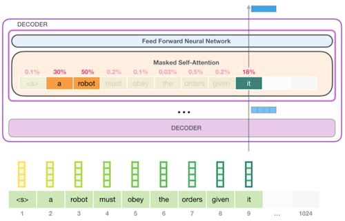
12.4.3 Decoder-only: GPT
Improving language understanding with unsupervised learning 논문(2018)
대표적인 Decoder-only 모델인 GPT는, 비지도 사전학습 단계의 objective로 다음 단어를 예측한다. (next word prediction)
- $\mathcal{U} = \lbrace u_1, \cdots, u_n \rbrace$ : unsupervised corpus of tokens
$$ L_1(\mathcal{U}) = \sum_{i} \log P (u_i | u_{i-k}, \cdots , u_{i-1}; \Theta) $$
다음은 GPT-2 학습에서 "a robot must obey the orders given it" 문장을 입력으로 주고, 다음 word를 예측한 예시다.
Notes: fine-tuning은 supervised learning으로 진행된다. (참고로 GPT-3 이상으로 큰 모델에서는 fine-tuning 없이, zero-shot/few-shot만으로 downstream tasks에 적용할 수 있다.)
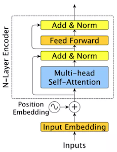
12.5 Absolute/Relative Positional Encoding
Self-Attention with Relative Position Representations 논문(2018)
가령 Absolute Positional Encoding를 통해 모델을 4K length 데이터로 학습했다고 가정하자. 사전학습된 모델에 만약 6K의 입력을 전달한다면 제대로 동작하지 않는 문제가 발생한다.
이러한 Absolute PE의 단점을 보완하기 위해, Relative Positional Encoding 기법이 새롭게 제안되었다. 해당 기법에서는 attention score에 Q, K 사이의 상대적인 위치 정보를 반영한다. (Value에는 직접적인 영향을 미치지 않음)
| Absolute PE | Relative PE | |
|---|---|---|
 |
 |
|
| Fusing | input embeddings(Q/K/V) + positional information |
attention score + relative distance information |
따라서 relative PE으로 학습한 모델은, 학습에서 본 적 없는 sequence length에 대해서도 generalization이 가능하다.
train short, test long 같은 활용도 가능하다. (단, 언제나 가능하지는 않음)
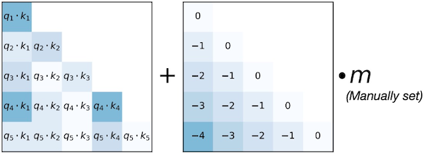
12.5.1 ALiBi: Attention with Linear Biases
Train Short, Test Long: Attention with Linear Biases Enables Input Length Extrapolation 논문(2021)
ALiBi 논문에서는 absolute index를 사용하지 않고, 오로지 relative distance만으로 positional encoding을 수행한다. (이를 통해 "train short, test long"을 가능하게 만든다.)
다음은 ALiBi 방법으로, attention matrix에서 offset(relative distance 정보)을 계산한 예시다.
12.5.2 RoPE: Rotary Positional Encoding
RoFormer: Enhanced Transformer with Rotary Position Embedding 논문(2021)
위 논문에서는 2D rotation을 기반으로 하는 positional embedding을 제안하였다. (참고로 RoPE는 LLaMA 모델에서 사용된다.)
(1) 임베딩 차원 $d$ 를 $d/2$ 쌍으로 분리한다. (각 쌍은 2차원의 한 축을 담당)
(2) position $m$ 에 따라 rotation을 적용한다. (임베딩은 복소수 타입으로 변환된다.)
$$ \Theta = \lbrace {\theta}_i = {10000}^{-2(i-1)/d}, i \in [1, \cdots, d/2] \rbrace $$
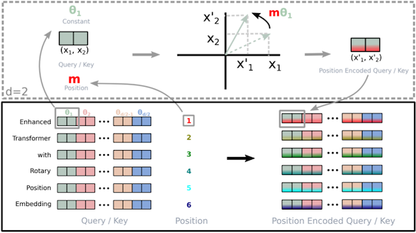
10000: 모든 token을 구분할 만큼 충분히 큰 상수
이를 general form으로 표현하면 다음과 같다.
$$ f_{q,k}(x_m, m) = R_{\Theta, m}^d W_{q,k}x_m $$
$$ R_{\Theta, m}^d = \begin{bmatrix} \cos(m \theta_1) & -\sin(m \theta_1) & 0 & 0 & \cdots & 0 & 0 \ \sin(m \theta_1) & \cos(m \theta_1) & 0 & 0 & \cdots & 0 & 0 \ 0 & 0 & \cos(m \theta_2) & -\sin(m \theta_2) & \cdots & 0 & 0 \ 0 & 0 & \sin(m \theta_2) & \cos(m \theta_2) & \cdots & 0 & 0 \ \vdots & \vdots & \vdots & \vdots & \ddots & \vdots & \vdots \ 0 & 0 & 0 & 0 & \cdots & \cos(m \theta_{d/2}) & -\sin(m \theta_{d/2}) \ 0 & 0 & 0 & 0 & \cdots & \sin(m \theta_{d/2}) & \cos(m \theta_{d/2})\end{bmatrix} $$
12.5.3 Advantage of RoPE: Extending the Context Window
Extending Context Window of Large Language Models via Position Interpolation 논문(2023)
대부분의 LLM은 제한된 context length 설정으로 학습된다. 예를 들어 LLaMA는 2k, LLaMA-2는 4k, GPT-4는 8k로 학습되었다.
하지만 interpolating RoPE를 통해, 이러한 context length 제한을 극복할 수 있다. (논문에서는 LLaMA를 2k에서 32k로 확장)
interpolation: 정수 인덱스에 0.5 인덱스를 추가하여, 1, 1.5, 2, 2.5, 3, ... 과 같이 확장하는 것을 의미한다.
주파수를 반으로 줄인 예시( ${\theta}_i/2$ )를 살펴보면, 기존에 대비해 동일한 범위에서 더 많은 성분을 갖고 4k position까지 표현하는 것을 확인할 수 있다.
| Conventional | 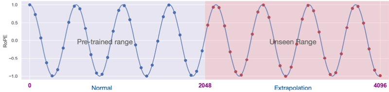 |
$m \in [0, 2048 * 2), {\theta}_i' = {\theta}_i$ |
| Interpolating | 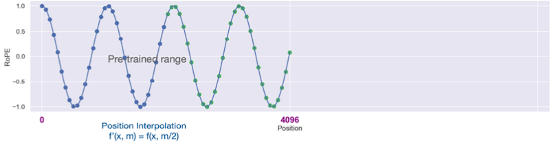 |
$m \in [0, 2048 * 2), {\theta}_i' = {\theta}_i/2$ |
12.6 KV Cache Optimizations
decoding(GPT-style)의 attention 계산에서는, 대체로 이전의 모든 Key, Value를 저장해 두는 방식으로 수행된다. (KV cache)
다음은 세 개의 토큰을 입력으로 갖는 masked self-attention을 나타낸 예시다. masked self-attention에서 새로운 query token은 이전 token이 보여야 한다.
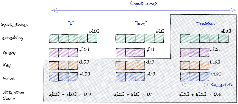
이때, 이전의 K, V 계산을 cache해 두는 것으로 동일한 계산을 반복할 필요가 없다.
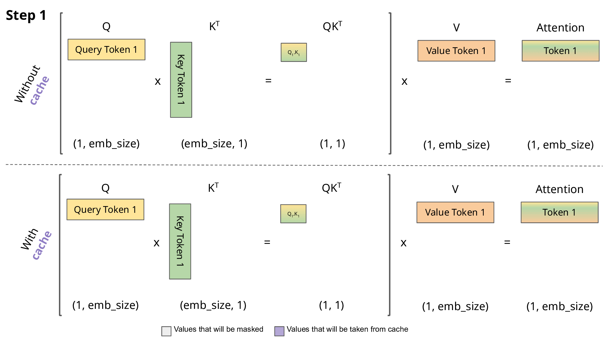
오로지 현재의 query token만 유지하면 되지만, 대신 보라색으로 표시된 부분을 메모리에 항상 유지해야 한다.
그러나 이러한 KV cache는, 유지를 위해서 굉장히 많은 메모리를 필요로 하게 된다. ( $2 \mathrm{bytes}$ = FP16 )
- Llama-2-7B, KV cache size
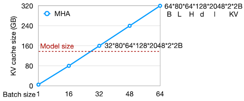
$$ \underset{minibatch}{BS} * \underset{layers}{32} * \underset{heads}{32} * \underset{n_{emd} }{128} * \underset{length}{N} * \underset{K,V}{2} * {2}\mathrm{bytes} = 512\mathrm{KB} \times BS \times N $$
- Llama-2-13B, KV cache size
$$ \underset{minibatch}{BS} * \underset{layers}{40} * \underset{heads}{40} * \underset{n_{emd} }{128} * \underset{length}{N} * \underset{K,V}{2} * {2}\mathrm{bytes} = 800\mathrm{KB} \times BS \times N $$
- Llama-2-70B, KV cache size
$$ \underset{minibatch}{BS} * \underset{layers}{80} * \underset{heads}{64} * \underset{n_{emd} }{128} * \underset{length}{N} * \underset{K,V}{2} * {2}\mathrm{bytes} = 2.5\mathrm{MB} \times BS \times N $$
가령 Llama-2-70B(using MHA) 학습 설정을 $BS=16$ , $n_{seq} = 4096$ 으로 가정하면, 필요한 KV cache size는 160GB가 된다. (A100 GPU 두 대가 필요한 수준)
Llama-2 paper 기준에서는 $BS=1$ $n_{seq} = 4096$ 으로 10GB의 메모리를 필요로 하였다.
다음 그래프에서는 batch size의 증가에 따라, KV cache size가 선형적으로 증가하는 것을 확인할 수 있다.
12.6.1 Multi-Query Attention (MQA)
Fast Transformer Decoding: One Write-Head is All You Need 논문(2019)
GQA: Training Generalized Multi-Query Transformer Models from Multi-Head Checkpoints 논문(2023)
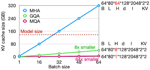
위 논문에서는 KV cache size를 줄이기 위해, #kv-heads 수를 최적화할 수 있는 방법을 제시하였다. 다음은 $N$ heads for query 조건에서 세 가지 설계를 비교한 도표이다.
| Multi-head | Multi-query | Grouped-query | |
|---|---|---|---|
 |
 |
 |
|
| #heads for K, V | $N$ | 1 | $G$ |
보편적으로 $G = N/8$ 로 설정하면, 정확도를 유지하면서 KV cache size를 줄일 수 있다.
- 세 가지 설계에서 KV cache size를 비교하면 다음과 같다.
- Accuracy
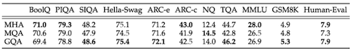
다음은 Llama-2, 30B, 150B tokens 설정에서, 각 설계의 정확도를 비교한 도표다.
12.7 Gated Linear Units (GLU)
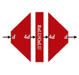
vanilla FFN을 GLU(Gate Linear Unit)로 변경하는 것으로도 성능을 향상시킬 수 있다. 3번의 matrix multiplication을 포함하며, activation function으로 swish를 사용한다.
$$ \mathrm{FFN_{SwiGLU} }(x, W, V, W_2) = (\mathrm{Swish_1}(xW) \otimes xV)W_2 $$
| FFN | SwiGLU |
|---|---|
 |
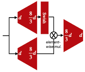 |
total computing cost를 유지하기 위해 $8/3d$ 차원으로 설정하였다.