Lecture 17 - TinyEngine - Efficient Training and Inference on Microcontrollers
Lecture 17 - TinyEngine - Efficient Training and Inference on Microcontrollers | MIT 6.S965
EfficientML.ai Lecture 11 - TinyEngine and Parallel Processing (MIT 6.5940, Fall 2023, Zoom)
17.4 SIMD Programming
ARM Cortex-M4, M7를 포함한 다양한 프로세서에서는, 명령어를 병렬로 수행할 수 있는 SIMD(Single Instruction Multiple Data) 명령어를 지원한다.
| Single Instruction Single Data | Single Instruction Multiple Data(SIMD) | |
| Desc | 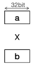 | 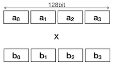 |
| Code |
|
|
| \#Ops | $N^3$ | $N^3/4$ |
17.4.1 ARM Cortex-M: CMSIS-NN Kernels
CMSIS-NN: Efficient Neural Network Kernels for Arm Cortex-M CPUs 논문(2018)
Cortex-M 프로세서에서는, dual 16-bit Multiply-and-Accumulate 명령어(SMLAD)를 비롯한 다양한 SIMD 명령어를 지원한다. (모든 레지스터는 32-bit wide로 구성)
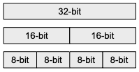
2 x INT16혹은4 x INT8SIMD 연산 지원
17.4.1.1 Example: 16-bit MAC Instruction
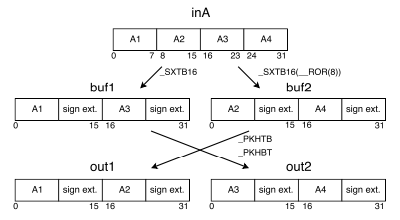
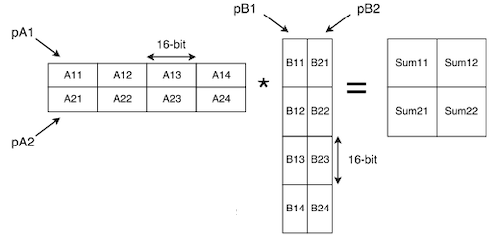
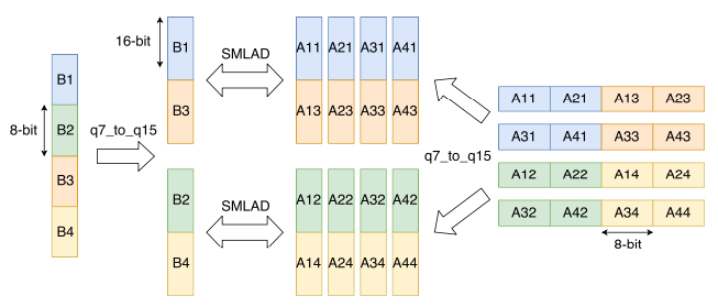
수많은 신경망 연산 함수에서 16-bit MAC 명령어를 활용한다. 다음은 INT8 양자화를 가정했을 때, 16-bit SMLAD 명령어가 수행되는 과정을 보여준다.
(1) 8-bit to 16-bit sign-extension
-
ROR: rotate right -
SXTB16: sign extend and pack to 16 bits -
PKHTB: pack high half to bottom,PKHBT: pack high to bottom
|  |
|
입력과 가중치 모두
q7_t타입일 경우, 별도의 재정렬이 필요하지 않다.offline에서 가중치를 미리
SMLAD에 최적화된 정렬로 재배치해둘 수 있다. (e.g., 입력이q15_t타입인 경우)
(2) Matrix multiplication
SMLAD: signed multiply accumulate dual
|  |
|
17.4.1.2 Example: Fully Connected Layer
fully-connected layer 연산의 배치 크기는 1이므로, 이때의 주된 연산은 matrix-vector multiplication에 해당된다.
- 1 loop iteration: 2개의 1x4 MAC 연산 수행
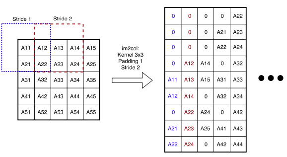
17.5 Im2col Convolution
Im2col이란, 입력 이미지 텐서를 columns 데이터로 변환하는 기법이다. (대표적으로 GEMM 행렬 곱셈을 위해 사용) 다음은 3차원 입력 이미지를 대상으로, direct convolution과 im2col convolution 과정을 비교한 예시다.
-
Direct: 6개의 중첩 반복문
-
Im2col: 3개의 중첩 반복문
| Conv | Description |
|---|---|
| Direct | 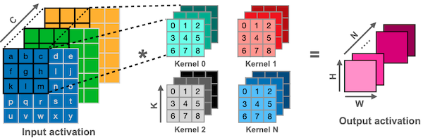 |
| Im2Col | 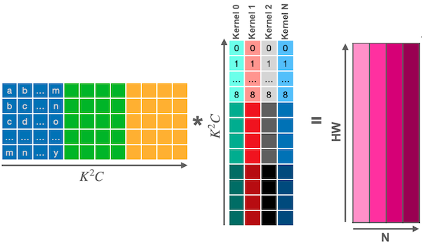 |
하지만 column마다 중복되는 데이터를 가지게 되면서, 이전보다 많은 메모리 공간을 차지하게 된다.
메모리 문제를 해결하기 위해 implicit GEMM 기법을 사용한다.
Notes: 2D 입력 이미지 im2col 예시
17.6 In-place Depth-wise Convolution
In-place 연산은 입력 데이터의 메모리 공간에, 출력 데이터를 write back으로 덮어쓰는 메모리 최적화 기법이다.
다음은 Inverted bottleneck 구조의 peak memory 사용량을 줄이기 위한, In-place depth-wise convolution을 나타낸 그림이다. (임시 버퍼 활용)
| General depth-wise convolution | In-place depth-wise convolution |
|---|---|
 |
 |
| peak memory: $2 \times C \times H \times W$ | peak memory: $(1 + C) \times H \times W$ |
17.7 How to Choose the Appropriate Data Layouts
다음은 두 convolution 연산(pointwise, depthwise)에서, NHWC 및 NCHW 데이터 레이아웃 방식을 비교한 표다.
| Conv | Description | Layout |
|---|---|---|
| pointwise | 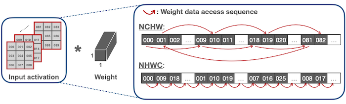 |
NHWC |
| depthwise | 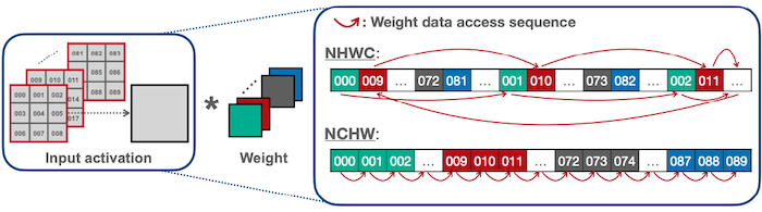 |
NCHW |
17.8 Winograd Convolution
다음은 direct convolution과 Winograd convolution의 계산 과정을 비교한 그림이다.
| Conv | Description |
|---|---|
| Direct |  |
| Winograd | 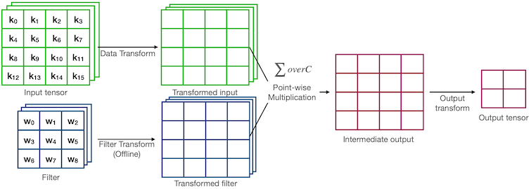 |
예제에서 연산량(MACs for 4 outputs)은 다음과 같다.
Direct = $9 \times C \times 4$
Winograd = $16 \times C$ (2.25x 감소)
17.8.1 Example: Formula for 3x3 Convolution
Winograd convolution은 다음과 같은 변환 트릭을 포함하는 수식으로 표현된다.
$$ Y = \overset{Output \ Transform}{A^T}[\underset{Filter \ Transform}{[GgG^T]} \odot\underset{Data \ Transform}{[B^TdB]}] \ A $$
$g$ : 3x3 filter, $d$ : input tile
이때 Transform 종류에 따라 offline 혹은 online 시점에 계산된다.
(1) Online
- Output Transform
$A^T = \begin{bmatrix} 1 & 1 & 1 & 0 \ 0 & 1 & -1 & -1 \end{bmatrix}$
- Data Transform $V$
$B^T = \begin{bmatrix} 1 & 0 & -1 & 0 \ 0 & 1 & 1 & 0 \ 0 & -1 & 1 & 0 \ 0 & 1 & 0 & -1 \end{bmatrix}$
$B = \begin{bmatrix} 1 & 0 & 0 & 0 \ 0 & 1 & -1 & 1 \ -1 & 1 & 1 & 0 \ 0 & 1 & 0 & -1 \end{bmatrix}$
(2) Offline
- Filter Transform $U$
$G = \begin{bmatrix} 1 & 0 & 0 \ 1/2 & 1/2 & 1/2 \ 1/2 & -1/2 & 1/2 \ 0 & 0 & 1 \end{bmatrix}$
$G^T = \begin{bmatrix} 1 & 1/2 & 1/2 & 0 \ 0 & 1/2 & -1/2 & 0 \ 0 & 1/2 & 1/2 & 1 \end{bmatrix}$