Lecture 16 - On-Device Training and Transfer Learning (Part II)
Lecture 16 - On-Device Training and Transfer Learning (Part II) | MIT 6.S965
EfficientML.ai Lecture 21 - On-device Training (Zoom Recording) (MIT 6.5940, Fall 2024)
16.2 Compilers, Languages and Optimizations for DL
16.2.1 Example: Tensor Programming
다음은 가우시안 블러 C++ 코드를 최적화한 예시다.

| **Clean C++** (**9.94 ms** per megapixel) | **Fast C++** (**0.90 ms** per megapixel) |
|
|
100배의 속도 향상(9.94ms $\rightarrow$ 0.90ms)을 얻었지만, 텐서 프로그래밍의 난이도가 높고 가독성이 떨어진다.
16.2.2 Halide: Decoupling Computation and Scheduling
Decoupling algorithms from schedules for easy optimization of image processing pipelines 논문(2012)
Halide는 알고리즘과 스케줄링을 분리한 도메인 특화 언어(Domain-Specific Language, DSL)로, 이미지 처리(특히 block convolution) 최적화를 위해 제안되었다.
다음은 Halide로 local Laplacian 필터를 정의한 코드 예시다.
-
Algorithm: 수평, 수직 3x3 blur 필터 정의
-
Schedule: 병렬 처리 정의
|  |
|
코드 크기 비교: Adobe 필터 1500줄 vs. Halide 필터 60줄 (c.f., Halide가 기존 Adobe 필터 대비 2배 빠르다.)
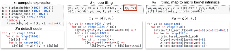
16.2.3 TVM: Learning-based DL Compiler
TVM: An Automated End-to-End Optimizing Compiler for Deep Learning 논문(2018)
TVM은 다양한 하드웨어 대상으로 딥러닝 application을 최적화하는 데 특화된 컴파일러다. (하드웨어별 최적화에 있어서, 엔지니어링 비용의 최소화)
다음은 MatMul 연산을 TVM의 Tensor Expression 언어로 나타낸 예시다.
Halide의 연산/스케줄 분리 정책을 따른다.
C = tvm.compute(
    (m, n),
    lambda y, x: tvm.sum(A[k, y] * B[k, x], axis=k)
)
Tensor IR은 최종적으로 하드웨어 명령어로 매핑된다.
| **Vanilla Code Generation** |
|
| **Loop Tiling for Locality** |
|
| **Map to Hardware Instructions** |
|
16.2.3.1 Example: Tensor Index Expression
- Compute C = dot(A, B.T)
import tvm

m, n, h = tvm.var('m'), tvm.var('n'), tvm.var('h')
A = tvm.placeholder((m, h), name='A')     // Input
B = tvm.placeholder((n, h), name='B')

k = tvm.reduce_axis((0, h), name='k')
C = tvm.compute((m, n),                   // C shape
      lambda i, j: tvm.sum(A[i, k] * B[j, k], axis=k)) // Computation Rule
- Convolution
out = tvm.compute((c, h, w),
 lambda i, x, y: tvm.sum(data[kc,x+kx,y+ky] * w[i,kx,ky], [kx,ky,kc]))
- ReLU
out = tvm.compute(shape, lambda *i: tvm.max(0, out(*i)))
16.2.3.2 Example: Schedule Transformation
예를 들어, 다음과 같이 연산을 정의했다고 하자.
|
|
- split
|
|
- reorder
|
|
- CUDA binding
|
|
16.2.3.3 Example: Tensor Instruction
w, x = t.placeholder((8, 8)), t.placeholder((8, 8))
k = t.reduce_axis((0, 8))
y = t.compute((8, 8), lambda i, j:
               t.sum(w[i, k] * x[j, k], axis=k))    # 연산 정의

# hw intrinsic를 생성하기 위한 lowering rule
def gemm_intrin_lower(inputs, outputs):
    ww_ptr = inputs[0].access_ptr("r")
    xx_ptr = inputs[1].access_ptr("r")
    zz_ptr = outputs[0].access_ptr("w")
    compute = t.hardware_intrin("gemm8x8", ww_ptr, xx_ptr, zz_ptr)
    reset = t.hardware_intrin("fill_zero", zz_ptr)
    update = t.hardware_intrin("fuse_gemm8x8_add", ww_ptr, xx_ptr, zz_ptr)
    return compute, reset, update

gemm8x8 = t.decl_tensor_intrin(y.op, gemm_intrin_lower)
Notes: Compute Primitives
Scalar Vector Tensor
16.2.4 AutoTVM: Learning to Optimize Tensor Programs
그러나, 스케줄링 정책을 결정하려면 굉장히 큰 설계 공간을 탐색해야 한다. AutoTVM에서는 이러한 단점을 해결하기 위해, 설계 공간의 파라미터를 학습하여 최적화한다.
- e.g., 루프 타일링 크기
(ty, tx)
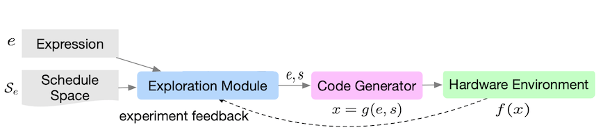
다음은 프레임워크의 세부 흐름도다. (cost model을 학습)
 |
 |
| No. | Description |
|---|---|
| (1) | surrogate model(e.g., Gaussian Process)을 활용해 $x^{\ast}$ 스케줄 선택 |
| (2) | $f(x^{\ast})$ 평가 |
| (3) | $(x^{\ast}, f(x^{\ast}))$ 를 데이터셋에 추가 |
| (4) | 모델을 데이터에 fit |
| (5) | 새로운 샘플 대상으로 (1)부터 반복 |
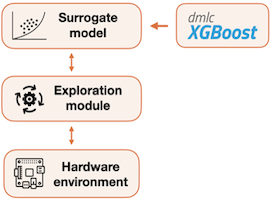
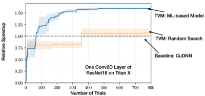
Notes: ML 기반 예측 성능 비교
16.3 Graph-level Optimization
단일 연산자 내부의 병렬성에서 더 나아가, 그래프 레벨에서 device utilization을 향상시키는 프레임워크가 제안되었다.
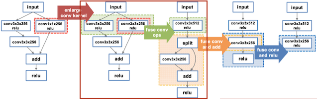
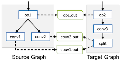
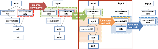
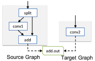
16.3.1 MetaFlow: Optimizing DNN Computation
MetaFlow: Optimizing DNN Computation with Relaxed Graph Substitutions 논문(2019)
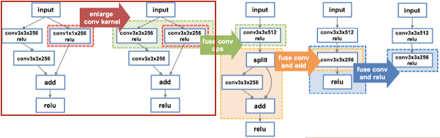
MetaFlow는 정확도를 유지하면서 연산량, 메모리 사용량 및 커널 호출 오버헤드를 줄일 수 있는 그래프를 탐색한다.
-
Enlarge Kernel: 연산량 늘지만, 커널 호출 감소 (수학적으로는 동일)
-
Fusion: 커널 호출 감소
 |
 |
 |
 |
 |
 |
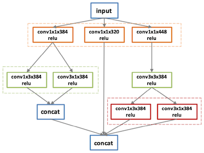
하드웨어별로 subgraph 지연시간 룩업 테이블을 기록하고, 탐색에서 활용한다.
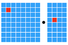
다음은 다양한 하드웨어에 맞춰 최적화한 그래프 예시다.
| Original | V100 | K80 |
|---|---|---|
 |
 |
 |
최종 그래프: V100 기준 30% 속도 향상
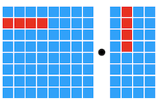
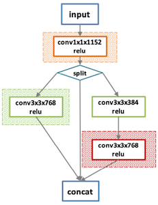
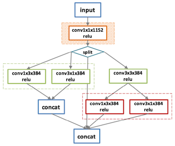
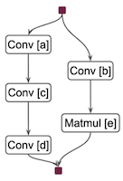
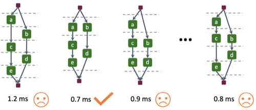
16.3.2 IOS: Inter-Operator Scheduler for CNN Acceleration
위 논문에서는 여러 연산자 간 병렬 스케줄을 탐색하는 IOS 프레임워크를 제안하였다. 다음은 연산 그래프를 최적화하는 예시다.
-
Merge: conv
a,b병합 -
Parallel: 연산을 두 그룹(
{c,d},{e})으로 분할하여 병렬 실행
| Sequential | Parallel, Merged |
|---|---|
 |
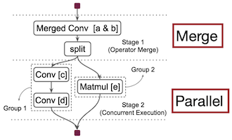 |
a->b->c->d->e |
a & b=>{c->d} & {e} |
서로 다른 그룹은 동시에 병렬로, 그룹 내부 연산은 순차적으로 실행된다.
하드웨어에 따른 최적 스케줄은, Dynamic Programming(DP) 기반으로 recursive하게 탐색한다.
-
알고리즘 시간 복잡도: $O((n/d+1)^{2d})$
-
연산자 집합 $S$ 의 지연시간 산출
= 이전 단계 최적 지연시간 $Latency[S-S']$ + 현재 단계 지연시간 $StageLatency[S']$
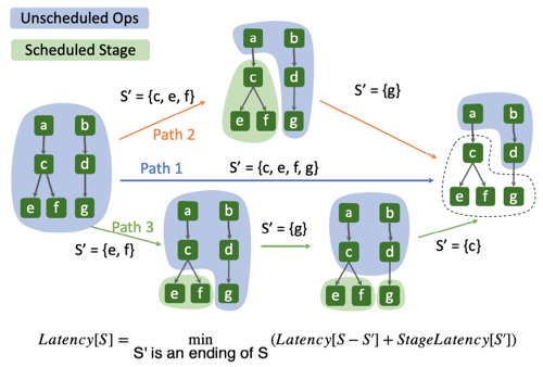
이때 지연시간은 실제 하드웨어에서 프로파일링한 값을 사용한다.
Notes: Specialized Scheduling 지원
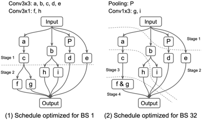
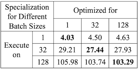
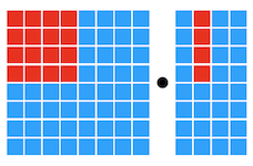
다음은 Inception V3 모델의 마지막 블록을, 여러 배치 크기(1, 32, 128) 설정에서 최적화한 그래프이다.
- bs = 32: 메모리 병목으로 인해 4 stage 구성
Schedule
(1 vs. 32)Latency(ms)
(1 vs. 32 vs. 128)