8 Neural Architecture Search (Part II)

Lecture 08 - Neural Architecture Search (Part II) | MIT 6.S965

Exploring the Implementation of Network Architecture Search(NAS) for TinyML Application

8.1 Performance Estimation in NAS

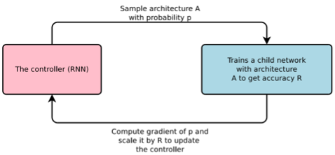
model architecture가 갖는 성능을 평가하는 방법을 생각해 보자. 우선 RNN controller를 쓰는 NAS는 다음과 같은 구조였다.

• probability $p$ 를 바탕으로 한 구조를 from scratch부터 학습시킨다.

• validation accuracy를 얻어서 controller를 update한다.

하지만 이러한 방법은 training cost가 너무 많이 든다.

8.1.1 Weight Inheritance

Net2Net: Accelerating Learning via Knowledge Transfer 논문(2015)

Efficient Architecture Search by Network Transformation 논문(2017)

모든 네트워크를 from scratch부터 학습시키기보다, weight를 상속하는 방법을 생각해 볼 수 있다. 작은 network를 weight inheritance를 사용하여 효율적으로 더 큰 네트워크를 구성한 Net2Net 논문이 대표적이다.

논문에서는 작은 모델을 teacher, teacher을 바탕으로 새롭게 만든 더 큰 모델을 student라고 부른다.

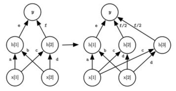
• Net2Wider

layer $i$ 의 hidden units $h[1], h[2]$ 에서 weights $c, d$ 를 복사하여 $h[3]$ unit을 추가한 예시다.

• 복사할 unit은 random하게 선택된다.

• 늘어난 unit 수만큼, $i+1$ 로 이어지는 연결에서는 넓어진 만큼 weight를 나눠서, 결과가 동일하도록 compensate한다.

  예제의 경우 $f/2$ 가 이에 해당된다.

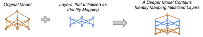
• Net2Deeper

identity mapping initization을 사용하여 capacity가 더 큰 네트워크를 만든다.

8.1.2 HyperNetwork: Weight Generator

SMASH: One-Shot Model Architecture Search through HyperNetworks 논문(2017)

Graph HyperNetworks for Neural Architecture Search 논문(2018)

SMASH 논문에서는 sampled model architecture가 가질 weight를 만드는 네트워크로 hypernetwork를 제시했다.(weight generator)

그렇다면 어떻게 weight를 만들어 낼 수 있을까? 우선 search space $\mathbb{R_c}$ 가 있다고 하자.

• 우선 HyperNet를 weights $H$ 로 initialize한다.

• loop를 수행한다.

training Error $E_t = f_c(W, x_i) = f_c(H(c), x_i)$ 를 구한 뒤 $H$ 를 update한다.

• input minibatch: $x_i$

• random architecture $c$

  해당 architecture가 가지는 weight는 $W = H(c)$ 이다.

• update한 $H$ 를 validation한다.

validation set $E_v = f_c(H(c), x_v)$ 를 구한다.

• random sample: $c$

8.1.3 Weight Sharing

Efficient Neural Architecture Search via Parameter Sharing 논문(2018)

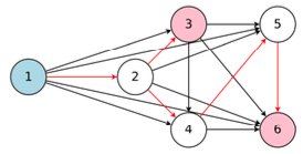
널리 쓰이는 다른 대표적인 방법으로는 weight sharing이 있다.

• 모든 graph를 포함하는 super-network를 학습한다.

• super-network에서 sub-graph를 추출하여 network architecture를 만든다.

• sub-network를 학습한다.

8.2 Performance Estimation Heuristics

하지만 몇 가지 방법은 network architecture training 없이, 오로지 구조를 관찰하여 performance estimation을 수행한다.

8.2.1 Zen-NAS

Zen-NAS: A Zero-Shot NAS for High-Performance Deep Image Recognition 논문(2021)

Gaussian complexity

Zen-NAS 논문에서는 Zen-Score라는 cost proxy를 도입하여 performance estimation을 수행한다. 오로지 random Gaussian input을 사용해 무작위로 초기화된 newtork에서, 몇 번의 forward inference를 수행하면 Zen-Score를 구할 수 있다.

• heuristic: 성능이 좋은 모델이라면 input perturbation에 sensitive할 것이다.

다시 말해 다른 입력들을 줬을 때 표준편차가 더 큰 모델을 찾으면 된다.

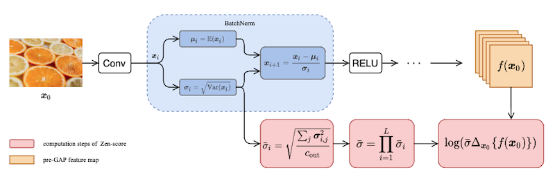
이러한 방식을 논문에서는 Zero-Shot NAS라고 부르며, Zen-NAS에서는 Batch Normalization으로 인해 발생할 수 있는 문제까지 고려한다. 다음은 Zen-Score를 구하는 과정을 나타낸 그림이다.

평균 $\mu$ , 분산 ${\sigma}^2$ 를 갖는 Gaussian distribution을 $\mathcal{N}(\mu, \sigma)$ 로 표현한다.

• $x_0$ : 입력 이미지 mini-batch 1개

• $x_i$ : $i$ 번째 레이어의 output feature map

• ${\sigma}_i$ : BN layer의 mini-batch deviation

• ${\triangle}_{x_0}\lbrace f(x_0) \rbrace$ : Global Average Pooling(GAP)을 거치기 전 feature map $f(x_0)$ 의 미분값(perturbation)

순차적으로 Zen-Score를 계산하는 방법을 살펴보자.

1. network $F(\cdot)$ 의 모든 residual links를 제거한다.

2. 모든 neurons(activations)이 $\mathcal{N}(0,1)$ 분포를 갖도록 weight를 초기화한다.

3. $\mathcal{N}(0,1)$ 에서 input $x$ 과 $\epsilon$ 을 sampling한다.

4. feature map perturbation $\triangle$ 을 계산한다.

$$ \triangle \overset{\triangle}{=} \mathbb{E_{x, \epsilon} } || f(x) - f(x+\alpha \epsilon)||_{F} $$

• $f: \mathbb{R^{m_0} } \rightarrow \mathbb{R^{m_L} }$

$L$ 개 레이어(function)을 의미한다.( $m_0$ : input dimension, $m_L$ : output dimension)

• $\alpha = 0.01$

• $\mathbb{E}$ : network expressivity(Gaussian complexity)

5. BN layer의 compensation term을 계산한다.

   output channels $m$ 개를 갖는 $i$ 번째 BN layer에서, 각 채널이 갖는 분산의 평균을 제곱근한 값을 계산한다.

$$ \bar{ {\sigma}{i} } = \sqrt{ {\sum} $$}{\sigma}^2_{i,j}/m

• ${\sigma}_{i,j}$ : $i$ 번째 BN layer의 $j$ 번째 output channel의 standard deviation.

6. Zen score를 계산한다.

$$ \mathrm{Zen}(F) \overset{\triangle}{=} \log(\triangle) + \sum_{i}\log(\bar{ {\sigma}_{i} }) $$

8.2.2 GradSign

GradSign: Model Performance Inference with Theoretical Insights 논문(2021)

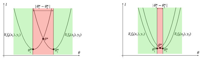
GradSign 논문에서는 다음과 같은 heuristic을 사용한다.

• heuristic: 다른 input sample을 줬을 때 각각의 local minima point의 distance가 작아야(denser) 성능이 좋은 모델이다.

• 좌측보다 우측이 denser sample-wise local optima를 갖는다. 즉, 우측이 더 성능이 좋은 모델이다.

• 다시 말해 그림의 빨간 영역을 최소화하여 최적의 구조를 찾을 수 있다.

8.3 Hardware-Aware NAS

다양한 hardware architecture에 알맞는 network architecture를 매번 검색한다면 엄청난 GPU cost가 발생할 것이다. 이러한 비용을 아끼기 위해 전통적으로는 proxy tasks를 utilize하는 방향으로 연구가 진행되었다.

다음은 몇 가지 예시이다.

• CIFAR-10에서 잘 동작하는 모델을 ImageNet에서도 잘 동작한다고 가정한다.

단점: 실제로는 capacity, complexity가 달라서 잘 동작하지 않는 경우가 많다.

• training epoch을 덜 진행한다.

단점: 일부 구조는 적은 epoch만으로도 빠르게 수렴한다.

• latency 대신 #Flops, #Parameters를 바탕으로 성능을 예측한다.

단점: #Flops가 적은 모델이라도 더 느릴 수 있다.

• small architecture space를 사용한다.

8.3.1 ProxylessNAS

ProxylessNAS: Direct Neural Architecture Search on Target Task and Hardware 논문(2018)

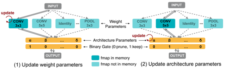
ProxylessNAS 논문은 proxy를 사용하지 않고 hardware에 알맞는 network architecture를 찾는다.

• 모든 candidate paths를 갖는 over-parameterized network를 구성한다.

• 학습은 over-parameterized network의 sigle training process로 구성된다.

만약 좋지 않은 path라면 해당 path를 pruning하면서 진행된다.

• architecture parameters를 binarize한 뒤, binary gate를 이용하여 오직 한 가지 path만 activate한다.

따라서 memory footprint가 작다.(O(N) $\rightarrow$ O(1))

그렇다면 latency는 어떻게 profile할까?

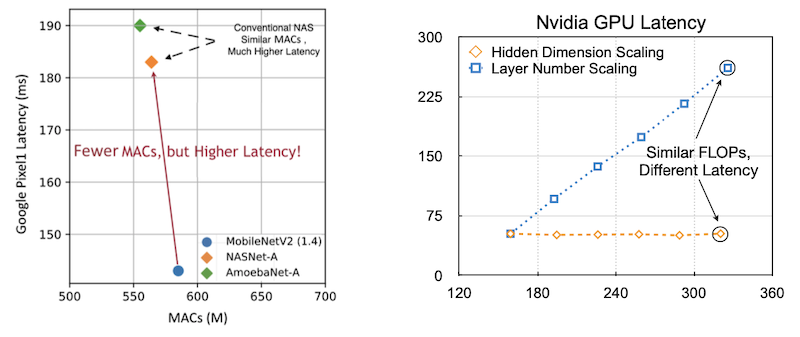
8.3.1.1 MACs is not a good metric for latency

우선 MACs와 Flops는 latency를 위한 proxy로 적합하지 않다.

• 왼쪽: MACs(x)-latency(y)

  MobileNetV2(파란색), NASNet-A(주황색), AmoebaNet-A(녹색)은 비슷한 수준의 MACs를 가지고 있지만, latency는 약 140ms, 180ms, 190ms로 차이가 크다.

• 오른쪽: FLOPs(x, M)-latency(y, ms)

  FLOPs는 비슷해도, 모델을 어떻게 scaling했는가에 따라 latency 차이가 크다.

  • 파란색: #layers를 줄였다.

  • 주황색: hidden dimension을 줄였다.

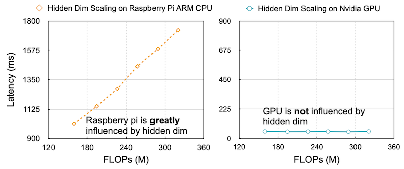
또한 hardware에 따라서도 scaling 방법 차이에 따라 latency 변화가 다르다.

• Raspberry Pi(ARM CPU): hidden dim이 늘어나면 동시에 latency가 늘어난다.

• GPU: hidden dim을 늘려도 GPU의 large parallelism 덕분에 크게 영향을 받지 않는다.

8.3.1.2 layer-wise latency profiling

따라서 ProxylessNAS에서는 latency predictor(지연시간 예측기)를 도입하여 latency를 예측한다.

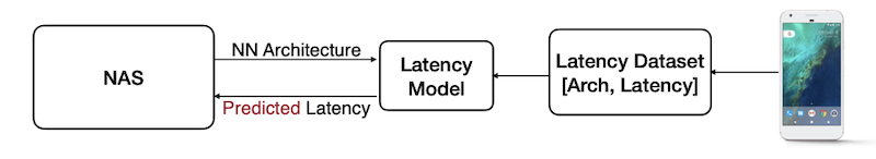
이때 latency predictor도 Lookup Table을 구성하는 단위에 따라서 layer-wise, network-wise로 나뉘는데, ProxylessNAS, Once-For-All에서는 layer-wise latency profiling을 사용한다.

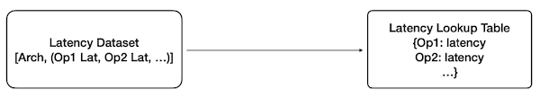
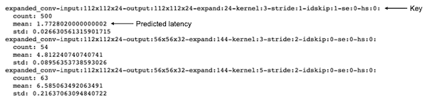
LUT 예시를 한 번 살펴보자.

• 첫 번째 줄 Key

  • 입력 차원 (112x112x24), 출력 차원 (112x112x24)

  • bottleneck layer의 출력 채널 24

  • kernel: 3x3

  • stride: 1

  • skip connection 사용(1), SE block 사용 X(0), h-swish 사용 X(0)

  h-swish를 사용하지 않는 경우 ReLU를 사용한다.

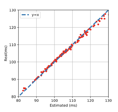
다음은 LUT를 사용한 latency predictor가 얼마나 latency를 예측하는지를 시각화한 그래프다.

8.3.2 HAT: network-wise latency profiling

HAT: Hardware-Aware Transformers for Efficient Natural Language Processing 논문

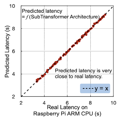
반면 HAT 논문에서는 network 단위로 latency profiling을 수행한다.

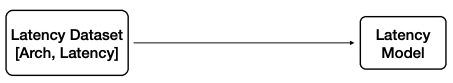
• [SubTransformer architecture, measured latency]

마찬가지로 시각화한 그래프를 보면 유효한 방법인 것을 알 수 있다.

8.3.3 Once-for-All NAS

Once-for-All: Train One Network and Specialize it for Efficient Deployment 논문(2019)

ONCE-FOR-ALL github

Once-for-All 논문에서는 supernet을 단 한 번 학습하면, 제약조건에 따라 다양한 subnet을 추출할 수 있는 방법을 제시한다.

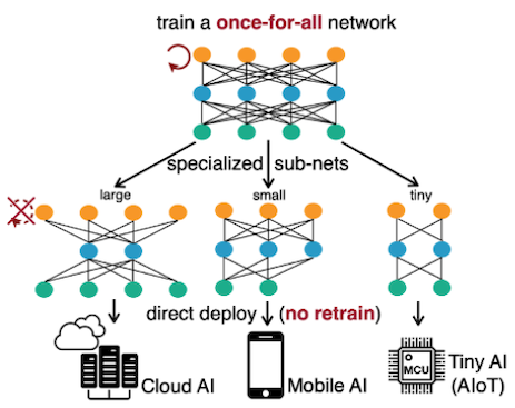
하지만 이러한 supernet training은 굉장히 큰 GPU cost를 필요로 한다. OFA에서는 Progressive Shrinking(PS)라는 접근법으로, 더 효율적으로 supernet training을 진행한다.

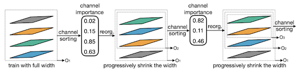
8.3.3.1 Progressive Shrinking

Progressive Shrinking은 다음과 같은 단계로 진행된다.

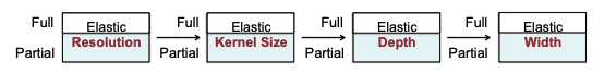
• Elastic Resolution

다양한 해상도 범위에서 제일 큰 구조를 학습한다.

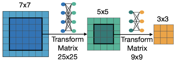
• Elastic Kernel Size

제일 큰 kernel size(7x7)가 아닌 5x5, 3x3 kernel size를 사용하는 구조를 학습한다.

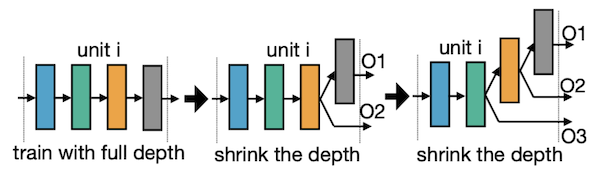
• Elastic depth

block에서 제일 많은 #layers(4개)가 아닌 3개, 2개 레이어를 갖는 구조를 학습한다.

• Elastic width

channel 중요도를 계산한 뒤, 중요하지 않은 channel을 pruning한다.