7 Neural Architecture Search (Part I)
Lecture 07 - Neural Architecture Search (Part I) | MIT 6.S965
AutoML은 크게 세 가지 process를 통칭하는 용어다. 이번 챕터는 그 중 Neural Architecture Search(NAS)에 대해 다룬다.
| feature engineering | Hyper-Parameter Optimization(HPO) | Neural Architecture Search |
|---|---|---|
| 도메인 지식에 기반한 feature engineering | hyperparameter의 meta-optimization | 최적 model architecture를 탐색 |
7.1 Basic Concepts
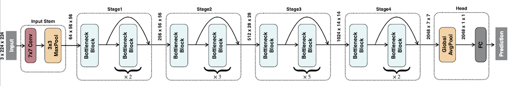
NAS는 모델 구조를 나누어 부를 때, 다음과 같이 input stem, stage, head 세 가지 용어를 주로 사용한다.
-
Input Stem
-
주로 큰 커널 크기( $7 \times 7$ )를 사용한다.
channel 수가 3개(RGB)로 적기 때문에, 계산량 자체는 적다.
-
Stage
-
출력 해상도가 동일한 block들의 집합이다. (first block에서 downsampling 수행)
-
downsampling이 있는 블록을 제외한, stage의 나머지 블록에서는 residual connection을 추가할 수 있다.
-
Head
-
application-specific하다. (detection head, segmentation head 등)
이때, early stage와 late stage의 특징을 비교하면 다음과 같다.
| early stage | late stage | |
|---|---|---|
| activation size | 크다 | 작다 |
| #parameters | 적다 | 많다 |
7.2 manually-designed neural network
다음은 ImageNet 데이터셋에서 학습한 여러 CNN 모델를, 연산량(MACs)-정확도 그래프에 나타낸 것이다.
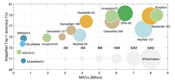
NAS는 이러한 CNN 모델에 기반하여, 더 효율적인 모델을 찾는 경우가 많다. 따라서, 먼저 이러한 CNN 모델을 살펴보자.
7.2.1 AlexNet, VGGNet
ImageNet Classification with Deep Convolutional Neural Networks 논문(2012): AlexNet
Very Deep Convolutional Networks for Large-Scale Image Recognition 논문(2014): VGGNet
다음은 CNN의 초기 모델인 AlexNet과 VGGNet의 구조를 비교한 도표다.
| AlexNet | VGGNet | |
|---|---|---|
| 구조 |  |
 |
| 특징 | ealry stage에서 큰 kernel size를 사용 ( $11 \times 11$ ) | early stage에서 작은 kernel을 여러 개 사용 ( $3 \times 3$ ) |
VGGNet에서는 $3 \times 3$ 레이어를 두 개 쌓는 것이, AlexNet보다 computational cost가 적게 들면서도 더 나은 성능을 보임을 입증했다.
- (-) 하지만 #layers, kernel call, memory access가 늘어나면서, 메모리 효율성 측면에서는 단점을 갖는다.

7.2.2 SqueezeNet: File Module
SqueezeNet: AlexNet-level accuracy with 50x fewer parameters and <0.5MB model size 논문(2016)
SqueezeNet은 $3 \times 3$ convolution을 fire module로 대체하여, 파라미터 수를 줄이면서 성능은 유지하여 효율적으로 연산을 수행한다.
| Architecture | Fire Module |
|---|---|
 |
 |
| head에서 GAP(Global Average Pooling)을 사용한다. | $1 \times 1$ convolution(squeeze), $3 \times 3$ convolution(expand)을 사용한다. |
fire module은 다음과 같은 단계로 연산이 진행된다.
| Squeeze | $\rightarrow$ | Expand | $\rightarrow$ | Concatenate |
|---|---|---|---|---|
| 채널 수를 줄인다. ( $1 \times 1$ ) | 채널 수를 확장한다. ( $1 \times 1$ , $3 \times 3$ ) | 출력을 합친다. |
7.2.3 ResNet50: Bottleneck Block
ResNet에서는 bottleneck block을 도입하여, 연산량은 줄이면서 residual connection을 통해 gradient vanishing 문제를 해결하며, 더 깊은 CNN 구조를 구현할 수 있게 되었다.
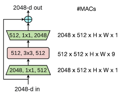
📝 예제 1: bottleneck block MACs
위 bottleneck block 그림에서 #MACs 연산이 얼마나 줄었는지 계산하라.
🔍 풀이
- full convolution(#channels 2048, #kernels 9)
$$ 2048 \times 2048 \times H \times W \times 9 = 512 \times 512 \times H \times W \times 144 $$
- bottleneck block
$$ 2048 \times 512 \times H \times W \times 1 $$
$$ + 512 \times 512 \times H \times W \times 9 $$
$$ + 2048 \times 512 \times H \times W \times 1 $$
$$ = 512 \times 512 \times H \times W \times 17 $$
총 8.5배 #MACs 연산이 줄어들었다.
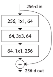
7.2.4 ResNeXt: Grouped Convolution
Aggregated Residual Transformations for Deep Neural Networks 논문(2017)
ResNeXt(2017) 논문은, grouped convolution을 도입하여 파라미터 수는 줄이면서 정확도는 늘렸다.
| ResNet(2015) | ResNeXt(2017) |
|---|---|
 |
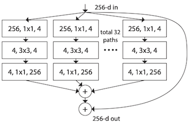 |
표기: #입력 채널 수, 필터 크기, # 출력 채널 수
논문에서는 group 수를 cardinality라는 용어로 정의한다.
7.2.5 ShuffleNet: 1x1 group convolution & channel shuffle
ShuffleNet: An Extremely Efficient Convolutional Neural Network for Mobile Devices 논문(2018)
ShuffleNet에서는, group convolution에서 channel information이 손실되는 것을 보완하기 위한 방법으로 channel shuffle을 제안했다.
| ShuffleNet block | Channel Shuffle |
|---|---|
 |
 |
7.2.6 SENet: Squeeze-and-Excitation Block
SENet은 Squeeze-and-Excitation(SE) block을 도입하여, feature map의 각 channel의 정보가 얼마나 중요한지를 판단한 뒤, 해당 채널을 강조하여 성능을 향상시킨다.
Transformer의 attention과 비슷한 메커니즘으로 볼 수 있다.
SE block은 다른 CNN model(VGG, ResNet 등)의 어디든 부착할 수 있다.
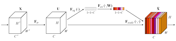
SE block은 Squeeze-Ecxcitation 두 단계로 이루어진다.
- Squeeze(압축)
global average pooling 연산을 이용하여, spatial information을 $1 \times 1$ 로 압축한다.(#channels $C$ 는 유지)
- $u_{c}$ : feature map( $H \times W$ )
$$ z = F_{sq}(u_{c}) = { {1} \over {H \times W} } {\sum_{i=1}^{H} }{\sum_{j=1}^{W} }{u_{c}(i, j)} $$
- Excitation(재조정)
squeeze된 벡터를 normalize한 뒤, 원래 feature map에 곱해준다. 이때 FC1 - ReLU - FC2 - Sigmoid 순서로 normalize된다.
-
$W_{1}, W_{2}$ : FC layer weight matrix
-
$\delta$ : ReLU 연산, $\sigma$ : Sigmoid 연산

$$ s = F_{ex}(z, W) = {\sigma}(W_{2} {\delta}(W_{1} z)) $$
이렇게 구한 가중치 벡터 $s$ 를 feature map $u$ 에 곱하는 것으로, 중요한 channel 값을 강조한다.
$$ F_{scale}(u_{c}, s_{c}) = s_{c} \cdot u_{c} $$
7.3 MobileNet Family
7.3.1 MobileNet: Depthwise-Separable Block
MobileNets: Efficient Convolutional Neural Networks for Mobile Vision Applications 논문(2017)
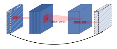
MobileNetV1(2017)은 depthwise, pointwise convolution 두 레이어가 연결된, depthwise-separable block을 제안했다.
input stem의 하나의 full conv을 제외하고, 나머지는 모두 depthwise-separable conv 연산으로 구성된다.
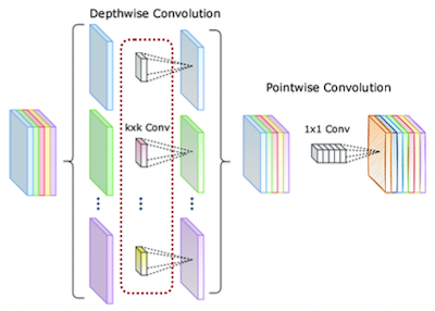
| depthwise conv | pointwise conv |
|---|---|
| 단일 채널마다 spatial information을 캡처 | spatial information을 mixing |
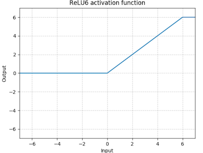
이때, conv 다음으로 이어지는 activation function(non-linearity)으로 ReLU6를 사용한다.
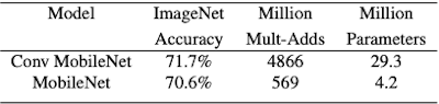
depthwise-separable block과 full conv block을 비교 시, 훨씬 적은 파라미터 수로 근소한 정확도를 확보한다.
depthwise-separable block: #channels = #groups인 극단적인 형태의 group convolution로도 볼 수 있다.
7.3.1.1 Width Multiplier, Resolution Multiplier
Width Transfer: On the (In)variance of Width Optimization 논문(2021)
MobileNet에서는 다양한 조건에 맞는 모델을 획득할 수 있도록, 두 가지 하이퍼파라미터를 추가로 사용한다.
| Width Multiplier $\alpha$ | Resolution Multiplier $\rho$ |
|---|---|
| 출력 채널 수에 적용 ( $N \rightarrow {\alpha}N$ ) | 입력 데이터의 해상도에 적용 |
$\alpha \in (0, 1]$ , $\rho \in (0, 1]$
7.3.2 MobileNetV2: inverted bottleneck block
MobileNetV2: Inverted Residuals and Linear Bottlenecks 논문(2018)
기존 bottleneck block의 문제점은, ReLU를 사용하면서 잃는 정보량이 많다는 점이다. MobileNetV2(2018)은 입력, 출력 채널 수를 늘리면, 정보 손실을 compensate할 수 있다는 아이디어로부터, inverted bottleneck block을 제안했다.
| inverted bottleneck block | stride=1 | stride=2 |
|---|---|---|
 |
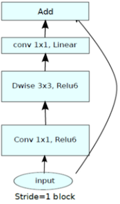 |
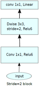 |
| block + residual connection | block + downsampling |
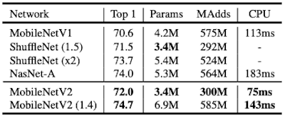
MobileNetV1과 비교했을 때, 더 적은 파라미터로 보다 우수한 성능을 획득했다.
7.3.3 MobileNetV3
MobileNetV3(2019)는 MobileNetV2의 후속 논문으로, NetAdapt algorithm + hardware-aware NAS를 이용해 찾은 개선된 architecture이다.
| MobileNetV3-Large | MobileNetV3-Small |
|---|---|
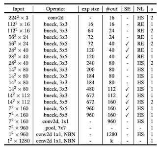 |
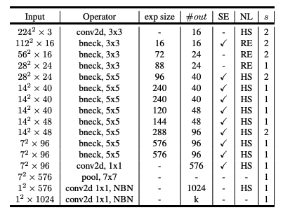 |
-
SE: Squeeze-and-Excitation block
-
NL: non-linearity
HS: h-swish, RE: ReLU
- NBN: no batch normalization
7.3.3.1 MobileNetV2 vs MobileNetV3
MbV3은 MbV2에서 비용이 큰 레이어(last stage)를 구조적으로 개선하고, 개선된 non-linearity function을 사용한다.
- redesign expensive layers
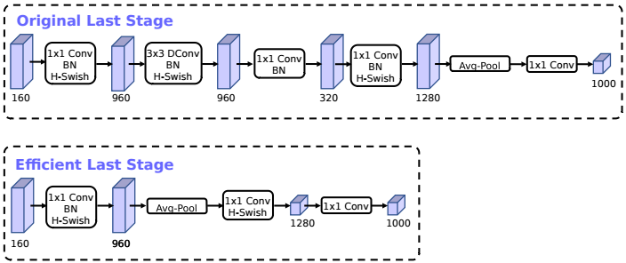
| MobileNetV2 | MobileNetV3 |
|---|---|
| 1x1 conv + avgpool (expensive) | avgpool + 1x1 conv (effective) |
- nonlinearity(activation function)
ReLU와 h-swish를 함께 사용한다. 미분해서 상수 값이 아니며, 일부 음수 값을 허용한다.
단독으로 h-swish만을 사용하기보다, ReLU와 함께 사용하면 더 좋은 성능을 보였다.
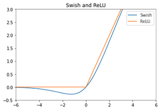
7.3.3.2 swish vs h-swish
swish는 sigmoid를 포함하기 때문에 복잡하고, 하드웨어 지원이 제한적이다. 이를 보완하기 위해 등장한 non-linearity가 바로 h-swish이다.
| ReLU vs swish | swish vs h-swish |
|---|---|
 |
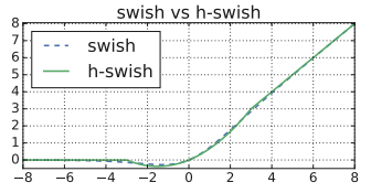 |
$$ \mathrm{swish} \ x = x \cdot {\sigma}(x) $$
$$ \mathrm{h} \ \mathrm{swish} \ = x{ {\mathrm{ReLU}6(x+3)} \over {6} } $$