Lecture 06 - Quantization (Part II)

Lecture 06 - Quantization (Part II) | MIT 6.S965

Neural Network Quantization Technique - Post Training Quantization

6.6 Quantization-Aware Training(QAT)

Quantization-Aware Training(QAT)이란 training 혹은 re-training(fine-tuning)을 통해, 최적의 quantization scheme을 찾는 방법이다.

	PTQ	QAT
속도	대체로 빠르다	느리다
re-training	불필요	필요
Plug and Play	가능	re-training 필요
accuracy drop	조절하기 힘들다.	어느 정도 조절할 수 있다.

Plug and Play(PnP): 별다른 설정없이 적용 가능

6.6.1 Simulated/Fake Quantization

모델의 학습 과정에서, 양자화 후 정확도를 미리 확인하는 simulation을 통해 최적의 양자화 정책을 결정할 수 있다. (simulated quantization = fake quantization)

훈련 중 weight W의 full precision copy는 유지된다.
정수 값을 사용하면 포착하지 못할 small gradient를 문제 없이 반영할 수 있다.
훈련 후 실제 추론에서는 quantized weight를 사용한다.

다음은 simulated quantization 방법을 통해, linear quantization 기반 weight, activation quantization을 수행하는 연산 그래프다.

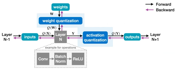
linear quantization forward, backward

Weight quantization

W \to S_{W} (q_{W} - Z_{W}) = Q (W)

Activation quantization

Y \to S_{Y} (q_{Y} - Z_{Y}) = Q (Y)

6.6.2 Straight-Through Estimator(STE)

Estimating or Propagating Gradients Through Stochastic Neurons for Conditional Computation 논문(2013)

UNDERSTANDING STRAIGHT-THROUGH ESTIMATOR IN TRAINING ACTIVATION QUANTIZED NEURAL NETS 논문(2019)

하지만 양자화된 값은 discrete하므로, 거의 대부분의 경우에서 미분 값은 0이 된다.

\frac{\partial Q (W)}{\partial W} = 0

따라서 다음과 같이 gradient update 과정 역시 불가능하게 된다.

g_{W} = \frac{\partial L}{\partial W} = \frac{\partial L}{\partial Q (W)} \cdot \frac{\partial Q (W)}{\partial W} = 0

이러한 문제를 해결하기 위해 등장한 방법이 Straight-Through Estimator(STE)이다.

$\partial Q (W) / \partial W$ deriative를 무시하고, identity function처럼 고려한다.
따라서 quantized weight만으로 바로 gradient update를 수행한다.

g_{W} = \frac{\partial L}{\partial W} = \frac{\partial L}{\partial Q (W)}

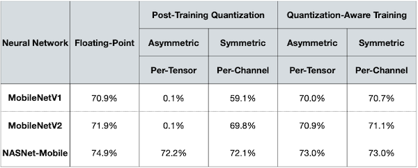
6.6.3 INT8 Linear Quantization-Aware Training

Quantizing deep convolutional networks for efficient inference: A whitepaper 논문(2017)

작은 모델에서는 INT8 linear QAT 방법이, PTQ보다 훨씬 더 좋은 정확도를 갖는 것을 알 수 있다.

QAT mobilenet

6.7 Binary Quantization

Binary Quantization은 더 나아가 1 bit만을 사용하는 양자화 방식이다.

storage: binary weights
computation: bit operation

real number weight 연산과, binary quantizated weight 연산을 비교해 보자.

baseline	Real Number Weights	Binary Quantized Weights

$y_{i} = \sum_{j} W_{i j} \cdot x_{j}$	$8 \times 5 + (- 3) \times 2 + 5 \times 0 + (- 1) \times 1$	$5 - 2 + 0 - 1$
operation	+ x	+ -
memory	1x	~32x less
computation	1x	~2x less

Binarization은 크게 deterministic binarization, stochastic binarizaion 방법으로 나뉜다.

Deterministic Binarization

정해둔 threshold 이상인 값은 1, 미만인 값은 -1로 양자화한다.(sign function)

q = s i g n (r) = {\begin{matrix} + 1, & r \geq 0 \\ - 1, & r < 0 \end{matrix}

Stochastic Binarization

global statistics 혹은 input data를 바탕으로, 양자화 시 -1, +1 probability를 결정한다.

6.7.1 Binarize the weights

BinaryConnect: Training Deep Neural Networks with binary weights during propagations 논문(2015)

대표적으로 BinaryConnection 논문은 다음과 같이 양자화한다.

discrete한 정도를 averaging할 수 있도록, hard sigmoid를 이용해서 probability를 결정한다.( $σ (r)$ )

hard sigmoid

q = {\begin{matrix} + 1, & w i t h p r o b a b i l i t y p = σ (r) \\ - 1, & w i t h p r o b a b i l i t y 1 - p \end{matrix}

σ (r) = min (max (\frac{r + 1}{2}), 1)

(-) 하지만 정확도 손실이 크다. (ImageNet 대상 AlexNet Top-1 accuracy: -21.2%p)
(-) 하드웨어에서 probability 계산을 위한 함수를 지원하지 않을 수 있다.

6.7.2 Binarize the weights with scaling factor

XNOR-Net: ImageNet Classification Using Binary Convolutional Neural Networks 논문(2016)

XNOR-Net 논문에서는 weight binarization에 따른 정확도를 회복하기 위해, binarized weight tensor(fp32)에 FP32 scaling factor를 추가한다.

W \approx α W^{𝔹}

weights (32bit float)	BinaryConnection	XNOR-Net

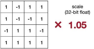이러한 scaling factor $α$ 는, 양자화 전 가중치 행렬 원소(FP32)의 절대값 평균을 사용한다.

α = \frac{1}{n} | | W | |_{1}

6.7.3 Binarize the weights and activations

혹은 weight과 activation에 모두 binary quantization을 적용할 수 있다. 이 경우 모든 연산을 XNOR 연산으로 대체할 수 있다. 가령 다음과 같은 연산을 생각해 보자.

y_{i} = \sum_{j} W_{i j} \cdot x_{j}

연산의 가능한 경우의 수는 다음과 같다.

W X Y=WX

1 1 1

1 -1 -1

-1 -1 1

-1 1 -1
-1 대신 0으로 바꾸면, XNOR 진리표와 완전히 일치한다.

$b_{w}$ $b_{x}$ XNOR( $b_{w}, b_{x}$ )

1 1 1

1 0 0

0 0 1

0 1 0

W	X	Y=WX
1	1	1
1	-1	-1
-1	-1	1
-1	1	-1

$b_{w}$	$b_{x}$	XNOR( $b_{w}, b_{x}$ )
1	1	1
1	0	0
0	0	1
0	1	0

앞선 예시와 비교 시, 메모리는 32배 이상, 연산은 58배 이상 줄어든다.

input	weight	operations	memory	computation
$ℝ$	$ℝ$	+ x	1x	1x
$ℝ$	$𝔹$	+ -	~32x less	~2x less
$𝔹$	$𝔹$	xnor, popcount	~32x less	~58x less

📝 예제 1: Binary Weight Quantization

다음 행렬 연산을 xnor 연산으로 계산하라.

binary quantization ex 4

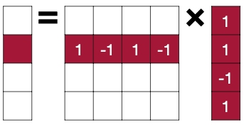
🔍 풀이

= 1 \times 1 + (- 1) \times 1 + 1 \times (- 1) + (- 1) \times 1 = - 2

= 1 x n o r 1 + 0 x n o r 1 + 1 x n o r 0 + 0 x n o r 1 = 1

하지만 단순히 -1을 0으로 치환해서는 다른 결과가 나오게 된다. 따라서 다음과 같은 보정을 거쳐야 한다.

1: 본래 -1, 1의 차이인 2를, 1의 개수만큼 더해준다.
0: -1을 치환한 값이므로, 0의 개수만큼 -1을 더해준다.

- 4 + 2 \times (1 + 0 + 0 + 0) = - 2

위 식을 다음과 같이 일반화할 수 있다.

y_{i} = - n + 2 \cdot \sum_{j} W_{i j} x n o r x_{j}

이는 원소 중 1의 개수가 얼마나 있는지를 파악하는, popcount 연산으로 대신할 수 있다.

y_{i} = - n + p o p c o u n t (W_{i} x n o r x) ≪ 1

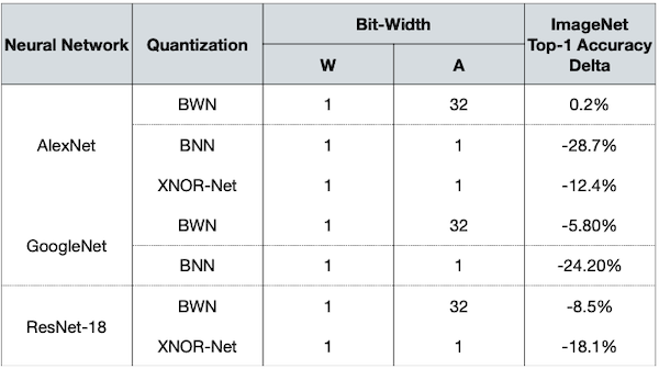
6.7.3 Accuracy Degradation of Binarization

다음은 다양한 binary quantization에 따른 정확도 변화를 정리한 도표이다.

BWN: scaling factor를 사용하는 Binary Weight Network
BNN: scale factors를 사용하지 않는 Binarized Neural Network

binary accuracy degradation

6.8 Ternary Quantization

Ternary Weight Networks 논문(2016)

1bit만을 사용하는 binary quantization보다 정확도를 보존하기 위해, 2bit(-1, 0, 1)를 사용한 quantization Ternary Weight Networks(TWN)가 등장했다.

q = {\begin{matrix} r_{t}, & r > △ \\ 0, & | r | \leq △ \\ - r_{t}, & r < - △ \end{matrix}

$△ = 0.7 \times 𝔼 (| r |)$
$r_{t} = E_{| r | > △} (r)$

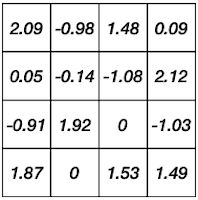
앞선 예시에 ternary quantization을 적용해 보자.

threshold $△$

△ = 0.7 \times \frac{1}{16} | | W | |_{1} = 0.73

scaling factor $r_{t}$

non-zero 값을 바탕으로 l1 norm을 계산한다.

\frac{1}{11} | | W_{W^{T} \neq 0} | |_{1} = 1.5

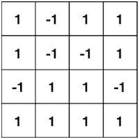
weights $W$ (32bit float)	ternary weights $W^{T}$ (2bit)

6.8.1 Trained Ternary Quantization(TTQ)

Trained Ternary Quantization 논문(2016)

Trained Ternary Quantization(TTQ) 논문에서는, 기존의 -1, 0, 1 대신 훈련 가능한 $w_{p}$ , $w_{n}$ 패러미터를 도입한 ternary quantization을 적용한다.

TTQ

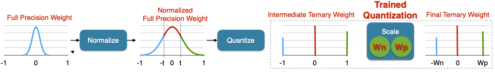
full precision 가중치를 [-1, 1] 사이로 normalize한다.
threshold에 따라 -1, 0, 1로 ternary quantization을 수행한다.
scale parameter $w_{n}$ , $w_{p}$ 를 훈련한다.

q = {\begin{matrix} w_{p}, & r > △ \\ 0, & | r | \leq △ \\ - w_{p}, & r < - △ \end{matrix}

다음은 ImageNet 대상 ResNet-18 모델에서, full precision, BWN, TWN 각각의 Top-1 accuracy를 비교한 도표다.

ImageNet Top-1 Accuracy	Full Precision	BWN(1 bit)	TWN(2 bit)	TTQ
ResNet-18	69.6	60.8	65.3	66.7