Lecture 05 - Quantization (Part I)
Lecture 05 - Quantization (Part I) | MIT 6.S965
EfficientML.ai Lecture 5 - Quantization (Part I) (MIT 6.5940, Fall 2023, Zoom recording)
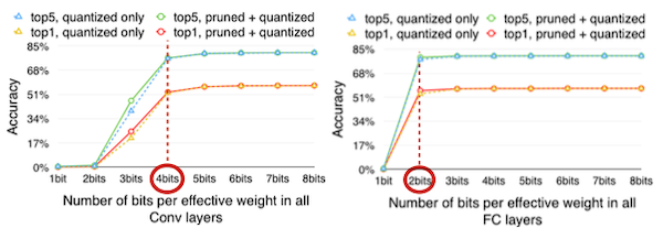
5.8 How Many Bits to Quantize Weights?
양자화를 위한 bit width는 어느 정도가 적당할까? 다음은 AlexNet의 Convolution, Fully-Connected 레이어에서, bit width 변화에 따른 정확도 변화를 나타낸 그래프다.
-
Conv layer: 4bits까지 정확도 유지
-
FC layer: 2bits까지 정확도 유지
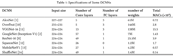
참고로 대표적인 CNN 모델에서 Conv, FC layer이 갖는 비중은 다음과 같다.
5.9 Deep Compression: Vector Quantization
Deep Compression 논문은 (1) iterative pruning, (2) vector quantization(VQ), (3) Huffman encoding 방법을 기반으로, 가중치가 차지하는 메모리를 획기적으로 줄이는 방법을 제안했다.
| Iterative Pruning | Vector Quantization(VQ) | Huffman Encoding | ||
|---|---|---|---|---|
 |
$\rightarrow$ |  |
$\rightarrow$ |  |
| original network 대비 크기 9x-13x 감소 |
original network 대비 크기 27x-31x 감소 |
original network 대비 크기 35x-49x 감소 |
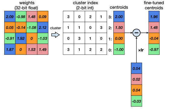
5.9.1 K-Means-based Weight Quantization
Deep Compression에서는 K-Means Algorithm 기반의, non-uniform weight quantization을 수행한다.(Vector Quantization)
#quantization levels = #clusters
Computer Graphics에서도 65536개의 스펙트럼으로 이루어진 원래 색상을, 256개 bucket을 갖는 codebook을 만들어서 유사하게 양자화한다.
-
storage: Integer Weights, Floating-Point Codebook
-
codebook: 예시 기준으로 FP32 bucket 4개를 사용한다.
-
cluster index: bucket이 4개이므로, 2bit(index 0,1,2,3)로 충분하다.
-
computation: Floating-Point Arithmetic
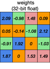
| Weights (FP32 x 16) |
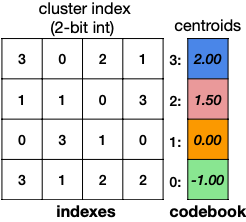
압축 | cluster index(INT2 x 16) centroids (FP32 x 4) |
추론 | Reconstructed (FP32 x 16) |
|---|---|---|---|---|
 |
→ |  |
→ | 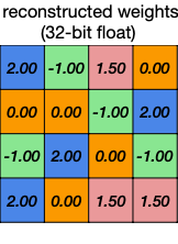 |
📝 예제 1: K-Means-based Quantization의 메모리 사용량
위 예시 그림에서 K-Means-based Quantization 이전/이후 사용하는 메모리 사용량을 계산하라.
🔍 풀이
- 양자화 전
FP32 $(4 \times 4)$ weight matrix
$$32 \ \mathrm{bits} \times (4 \times 4) = 512 \ \mathrm{bits} = 64 \ \mathrm{bytes} $$
-
양자화 후
-
weight matrix: INT2 x 16
$$2 \times (4 \times 4) = 32 \ \mathrm{bits} = 4 \ \mathrm{bytes} $$
- codebook: FP32 x 4
$$32 \times (1 \times 4) = 128 \ \mathrm{bits} = 16 \ \mathrm{bytes} $$
따라서 양자화 전 필요한 메모리 사용량은 64 bytes, 양자화 후 필요한 메모리 사용량은 20 bytes이다.(3.2배 사용량 감소)
weight tensor가 크면 클수록, 가중치의 메모리 사용량 감소 효과가 더 커진다.
5.9.2 Finetuning Codebook
위 예시에서 weight를 다시 reconstruct(decode)한 뒤, error를 계산해 보자.
| 양자화 전 | Decompressed | Error |
|---|---|---|
|
|
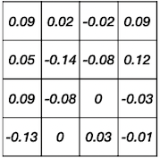 |
이러한 quantization error는 양자화 전, 후의 가중치 값 차이를 줄이는 방식으로, codebook을 fine-tuning하며 개선할 수 있다.
-
cluster index에 따라 quantization error를 분류한다.
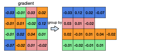
-
mean error를 구한다.
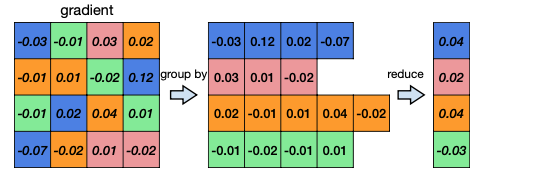
-
codebook의 centroid를 업데이트한다.
5.9.3 K-Means-based Quantization Limitations
그러나 K-Means-based weight quantization은 다음과 같은 한계점을 갖는다.
-
(-) 연산 시 다시 floating point로 reconstruct된다.
-
(-) reconstruction 과정에서 time complexity, computation overhead가 크다.
-
(-) weight가 메모리에서 연속적이지 않기 떄문에, memory access에서 긴 지연이 발생하게 된다.
-
(-) activation은 입력에 따라 dynamic하게 변하므로, activation quantization으로 clustering-based approach는 적합하지 않다.
5.9.4 Huffman Coding
추가로 Huffman Coding 알고리즘을 적용하여 memory usage를 더 줄일 수 있다.
Unix의 파일 압축, JPEG, MP3 압축에서 주로 사용된다.
Encoding의 분류는 크게 두 가지로 나뉜다. 고정된 길이로 encode하는 RLC(Run Length Coding), 가변 길이로 encode하는 VLC(Variable Length Coding). Huffman Coding은 대표적인 VLC에 해당된다.
-
frequent weights: bit 수를 적게 사용해서 표현한다.
-
In-frequent weights: bit 수를 많이 사용해서 표현한다.
📝 예제 2: Huffman Coding
a, b, c 알파벳을 Huffman Coding을 이용해 압축하라.
ASCII code로 표현하려고 한다면 INT8 x 3으로 24bits를 사용해야 한다. 하지만 Huffman coding을 적용하여 메모리 사용량을 줄일 수 있다.
🔍 풀이
a, b, c를 다음과 같이 압축하여 정의했다고 하자.
-
Try 1
a b c 01 101 010
$\rightarrow$ a와 c의 접두어 부분(01)이 겹치기 때문에 VLC로 압축할 수 없다.
-
Try 2
a b c 01 10 111
$\rightarrow$ 겹치는 접두어가 없기 때문에, 01 10 111 = 총 7bits로 압축할 수 있다.
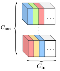
5.10 AND THE BIT GOES DOWN: Product Quantization
AND THE BIT GOES DOWN: REVISITING THE QUANTIZATION OF NEURAL NETWORKS 논문(2019)
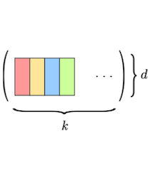
어떤 레이어가 $(C_{in} \times K \times K)$ 크기의 3D 텐서 $C_{out}$ 개를 갖는다고 하자. 위 논문에서는 합성곱 필터가 갖는 spatial redundancy를 이용할 수 있도록, $K \times K$ 크기를 갖는 subvector 단위로 vector quantization을 적용한다.
-
각 3차원 텐서를, subvector $C_{in}$ 개로 구성된 단일 벡터로 reshape한다.
-
subvector size $d$ : $K \times K$
-
#subvectors per vector: $C_{in}$
-
(크기 $d$ 를 갖는) subvector $k$ 개로 구성된 codebook 기반으로 양자화한다.
| Filters | Reshaped filters | Codebook |
|---|---|---|
 |
 |
 |
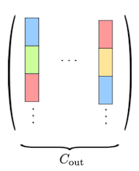
5.10.1 Product Quantization
앞서 살펴본 Vector Quantization(VQ)는 Product Quantization(PQ)의 특수한 경우로 볼 수 있다. 다음은 Product Quantization의 두 가지 경우를 비교한 표다.
| Vector Quantization | Scalar K-means algorithm | |
|---|---|---|
| subvector size $d$ | $C_{in}$ | $1$ |
| #subvectors per vector | $1$ | $C_{in}$ |
또한 product quantization에서 codebook $C = \lbrace c_1, \cdots , c_k \rbrace$ 는, 크기 $d$ 를 갖는 centroid(codeword) $k$ 개로 구성된다.
| Codebook | Codeword | |
|---|---|---|
 |
 |
|
| dimension | $d \times k$ | $d$ |
📝 예제 3: Product Quantization의 메모리 사용량
다음과 같은 조건에서 Product Quantization으로 사용되는 메모리 사용량을 계산하라.
-
입력 레이어: $(128 \times 128 \times 3 \times 3)$
-
#centroids: $k = 256$
데이터 타입은 float16을 사용하며, 각 subvector는 1 byte를 차지한다고 가정한다.
- block size: $d = 9$
🔍 풀이
메모리 사용량은 크게 (1) indexing cost와 (2) FP16 타입의 centroid가 차지하는 메모리로 나뉜다.
- indexing cost
입력 레이어의 #blocks $m$ 은 $128 \times 128 = 16,384$ 개다. 따라서 16kB 메모리를 차지한다.
- centroids
FP16을 사용하므로, 256개 centroids가 차지하는 메모리는 다음과 같다.
$$9 \times 256 \times 2 \ \mathrm{bytes} = 4,608 \ \mathrm{bytes}$$
5.10.2 Minimize Difference between Output Activations
최적의 centroid(codeword)를 찾기 위한 방법을 살펴보자. 먼저 양자화 전,후 가중치 값을 비교하며, quantization error를 최소화하는 objective function은 다음과 같이 정의할 수 있다.
$$ || W - \widehat{W}|{|}2^2 = \sum_2^2 $$} || w_j - q(w_j) |{|
- $q(w_j) = (c_{i_1}, c_{i_2}, \cdots , c_{i_m})$
하지만 논문에서는 양자화 전,후의 차이를 최소화해 얻은 가중치가, 반드시 양자화 전의 출력과 비슷한 결과를 보장하지 않는다는 사실에 주목한다. 대신 in-domain input을 추론시키면서, activation을 대상으로 양자화 전,후 차이를 최소화하는 objective function을 제안한다.
$$ || y - \widehat{y}|{|}2^2 = \sum_2^2 $$} || x(w_j - q(w_j)) |{|
다음은 개와 고양이를 분류하는 간단한 binary classifier $\varphi$ 를 대상으로, 두 가지 objective function을 사용한 결과를 비교한 그림이다.
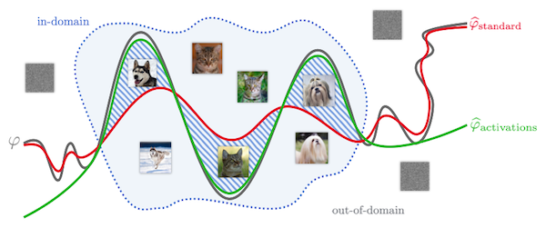
-
weight-based(빨간색), activation-based(초록색)
-
in-domain 입력에 대해, activation-based objective function으로 최적화한 모델의 성능이 더 우수하다.