Lecture 05 - Quantization (Part I)

Lecture 05 - Quantization (Part I) | MIT 6.S965

EfficientML.ai Lecture 5 - Quantization (Part I) (MIT 6.5940, Fall 2023, Zoom recording)

A White Paper on Neural Network Quantization

quantization(양자화)는 연속된 신호(입력)을 discrete set으로 변환하는 기술이다.

Before Quantization	After Quantization

메모리 사용량, 전력 소모, 지연시간, 하드웨어 설계(silicon area) 등 다양한 차원의 이득을 얻을 수 있다.

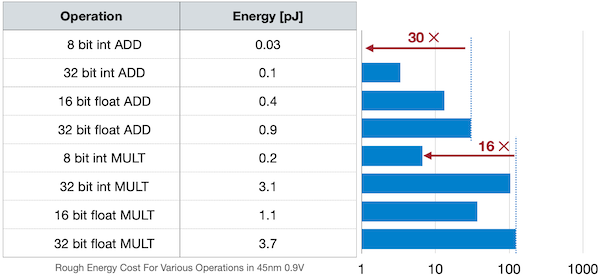
5.1 Numeric Data Types

대체로 bit-width를 사용하는 연산일수록, 에너지 소모량이 적어 효율적이다.

computation cost

5.1.1 Integer

다음은 십진수 49를 8 bit 정수(INT8)로 표현한 것이다.

Unsigned Integer n-bit range: $[0, 2^{n} - 1]$	![uint8 ex](https://github.com/erectbranch/MIT-Efficient-AI/blob/master/2022/lec05/summary01/images/int8_ex_1.png)
Signed Integer (Sign-Magnitude) n-bit range: $[- 2^{n - 1} - 1, 2^{n - 1} - 1]$ > $00000000_{(2)} = 10000000_{(2)} = 0$	![int8 sign-magnitude ex](https://github.com/erectbranch/MIT-Efficient-AI/blob/master/2022/lec05/summary01/images/int8_ex_2.png)
Signed Integer (Two's Complement Representation) range: $[- 2^{n - 1}, 2^{n - 1} - 1]$ > $00000000_{(2)} = 0$ , $10000000_{(2)} = - 2^{n - 1}$	![int8 two's complement ex](https://github.com/erectbranch/MIT-Efficient-AI/blob/master/2022/lec05/summary01/images/int8_ex_3.png)

5.1.2 Fixed-Point Number

fixed-point 표현은 정수 연산용으로 최적화된 하드웨어를 사용할 수 있다는 장점을 갖는다. 다음은 8bit fixed-point로 소수를 표현한 예시다.

핵심은 shift 연산이다. (shift right = 나누기 2, left shift = 곱하기 2)

`fixed<8,4>`(의미: Width 8bit, Fraction 4bit) - Sign(1bit) - Integer(3bit) - Fraction(4bit)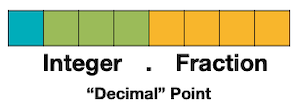

![fixed-point](https://raw.githubusercontent.com/erectbranch/MIT-Efficient-AI/master/2022/lec05/summary01/images/fixed-point.png)

다음은 unsigned fixed<8,3> 예시다.

00010.110 \underset{2}{} = 2 + 1 \times 2^{- 1} + 1 \times 2^{- 2} = 2 + 0.5 + 0.25 = 2.75 \underset{10}{}

5.1.3 Floating-Point Number (IEEE FP32)

다음은 IEEE 754 스타일의 32bit floating-point를 표현한 예시다.

Sign(1bit) Exponent(8bit) Fraction(mantissa, 23bit)

![32bit floating-point](https://github.com/erectbranch/MIT-Efficient-AI/blob/master/2022/lec05/summary01/images/fp32_ieee754.png)

(- 1)^{s i g n} \times (1 + F r a c t i o n) \times 2^{E x p o n e n t - 127}

Exponent Bias $= 127 = 2^{8 - 1} - 1$

e.g., IEEE FP32 0.265625 표현

$0.265625 = (1 + 0.0625) \times 2^{125 - 127} = 1.0625 \times 2^{- 2}$

5.1.3.1 Floating-Point Number: Subnormal Numbers

exponent 값이 0에 해당하는 범위를 subnormal number(비정규 값)라고 부른다.

fp32 ieee754 number range

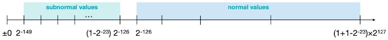
해당 영역은 normal number과 다르게 linear하다.

subnormal numbers

(- 1)^{s i g n} \times F r a c t i o n \times 2^{1 - 127}

Smallest $2^{- 149} = 2^{- 23} \times 2^{1 - 127}$	![subnormal number smallest](https://github.com/erectbranch/MIT-Efficient-AI/blob/master/2022/lec05/summary01/images/subnormal_smallest.png)
Largest $2^{- 126} - 2^{- 149} = (1 - 2^{- 23}) \times 2^{1 - 127}$	![subnormal number largest](https://github.com/erectbranch/MIT-Efficient-AI/blob/master/2022/lec05/summary01/images/subnormal_largest.png)

5.1.3.2 Floating-Point Number: Special Values

다음과 같은 두 가지 경우를 특수한 값으로 분류한다.

Infinity > Normal Numbers, Exponent $\neq$ 0	![fp32 infinity](https://github.com/erectbranch/MIT-Efficient-AI/blob/master/2022/lec05/summary01/images/subnormal_infty.png)
NaN (Not a Number) > Subnormal Numbers, Fraction $=$ 0	![fp32 NaN](https://github.com/erectbranch/MIT-Efficient-AI/blob/master/2022/lec05/summary01/images/subnormal_not_a_number.png)

5.1.4 Floating-Point Number Formats for Deep Learning

FP8 Formats for Deep Learning 논문(2022)

fraction와 exponent를 비교하면, 딥러닝에서는 exponent width가 더 중요하다.

다음 예시를 보면, half presicion(16bit) 기준에서 exponent width를 최대한 사용하려는 의도를 엿볼 수 있다.

Exponent (bits)	Fraction (bits)	Total (bits)
8	23	32
5	10	16
8	7	16

이후 NVIDIA에서는 FP8 format도 제안하였다.

	Exponent (bits)	Fraction (bits)	Total (bits)
	4	3	8
	5	2	8

5.1.5 INT4 and FP4

더 나아가 INT4, FP4 포맷도 등장하였다.

	Range (Positive Numbers)

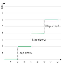
5.2 Uniform vs Non-uniform Quantization

$r$ : real value(원래 표현), $q$ : quantized value

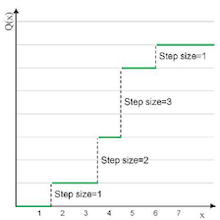
step size를 어떻게 정하는가에 따라 양자화를 분류할 수 있다.

	Uniform	Non-Uniform	Non-Uniform (Logarithmic)

장점	동일한 step size로 구현이 쉽다	표현력이 우수하다.	효율적으로 넓은 범위를 표현한다.

Uniform Quantization
$Z$ : Zero points, $S$ : Scaling factor

Q (r) = I n t (r / S) - Z

Non-Uniform Quantization

Q (r) = X_{i}, r \in [△_{i}, △_{i + 1})

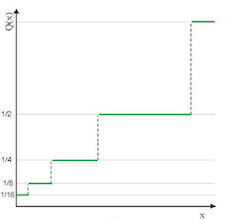
Non-Uniform Quantization: Logarithmic Quantization

Q (r) = S i g n (r) 2^{r o u n d (\log_{2} | r |)}

5.3 Linear Quantization

대표적인 uniform quantization에 해당하는 Linear Quantization을 살펴보자.

linear quantization mapping

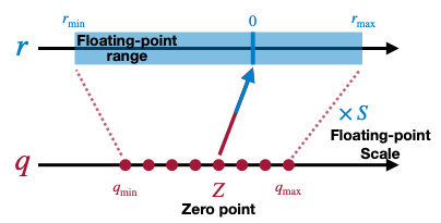
r = S (q - Z)

이때, floating-point range $r_{m i n}$ , $r_{m a x}$ , integer range $q_{m i n}$ , $q_{m a x}$ 는 이미 알고 있는 정보이다.

Bit Width	$q_{m i n}$	$q_{m a x}$
2	-2	1
3	-4	3
4	-8	7
N	$- 2^{N - 1}$	$2^{N - 1} - 1$

이를 바탕으로 양자화 scaling factor $S$ 및 zero point $Z$ 를 구할 수 있다.

S = \frac{r_{m a x} - r_{m i n}}{q_{m a x} - q_{m i n}}

위 식은, $r_{m a x} = S (q_{m a x} - Z)$ , $r_{m i n} = S (q_{m i n} - Z)$ 두 식을 연립하여 얻을 수 있다.

5.3.1 Example: 2-bit Linear Quantization

다음의 floating point 텐서를 2-bit 양자화해보자.

[\begin{matrix} 2.09 & - 0.98 & 1.48 & 0.09 \\ 0.05 & - 0.14 & - 1.08 & 2.12 \\ - 0.91 & 1.92 & 0 & - 1.03 \\ 1.87 & 0 & 1.53 & 1.49 \end{matrix}]

(1) scaling factor $S$

S = \frac{r_{m a x} - r_{m i n}}{q_{m a x} - q_{m i n}} = \frac{2.12 - (- 1.08)}{1 - (- 2)} = 1.07

(2) zero point $Z$

Z = q_{m i n} + \frac{r_{m i n}}{S} = r o u n d (- 2 - \frac{- 1.08}{1.07}) = - 1

Notes: 2-bit quantization

Binary Decimal

01 1

00 0

11 -1

10 -2

Binary	Decimal
01	1
00	0
11	-1
10	-2

5.3.2 Example: Matrix Multiplication

다음은 간단한 행렬 곱셈 수식이다.

Y = W X

양자화를 반영하면 다음과 같다.

S_{Y} (q_{Y} - Z_{Y}) = S_{W} (q_{W} - Z_{W}) \cdot S_{X} (q_{X} - Z_{X})

q_{Y}

에 대한 식으로 정리하면 다음과 같다.

q_{Y} = \frac{S_{W} S_{X}}{S_{Y}} (q_{W} - Z_{W}) (q_{X} - Z_{X}) + Z_{Y}

q_{Y} = \frac{S_{W} S_{X}}{S_{Y}} (q_{W} q_{X} - Z_{W} q_{X} - Z_{X} q_{W} + Z_{W} Z_{X}) + Z_{Y}

효율적으로 추론하기 위해, 가중치와 연관된 일부 항은 오프라인에서 미리 계산해 둔다.

$S_{W} S_{X} / S_{Y}$ : $N$ bit rescale
$+ Z_{Y}$ : $N$ bit addition

q_{Y} = \underset{r e s c a l e}{\frac{S_{W} S_{X}}{S_{Y}}} (q_{W} q_{X} - Z_{W} q_{X} \underset{P r e c o m p u t e}{- Z_{X} q_{W} - Z_{W} Z_{X}}) + Z_{Y}

5.3.3 Normalization of Multiplier

위 식에서 multiplier $M = S_{W} S_{X} / S_{Y}$ 는 (0,1) 값을 갖는다. 따라서, fixed-point 형태로 표현하는 것도 가능하다.

M = 2^{- n} M_{0}

$M_{0} \in [0.5, 1)$ : fixed-point multiplication
$2^{- n}$ : bit shift

fixed-point를 사용하면, $M_{0}$ 를 정수용 하드웨어로 연산할 수 있다.

5.4 Linear Quantized Neural Network Layers

가장 간단한 예제인 symmetric linear quantization을 살펴보자. ( zero point $Z = 0$ )

symmetric linear quantization

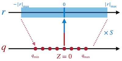
이때의 scaling factor $S$ 는 다음과 같다.

S = \frac{r_{m i n}}{q_{m i n} - 0} = \frac{- {| r |}_{m a x}}{q_{m i n}} = \frac{{| r |}_{m a x}}{2^{N - 1}}

위 식은 $r_{m i n} = S (q_{m i n} - Z)$ 에서 유도할 수 있다.

5.4.1 Fully-Connected Layer

이제 bias를 포함하는 fully-connected layer의 수식을 살펴보자.

Y = W X + b

S_{Y} (q_{Y} - Z_{Y}) = S_{W} (q_{W} - Z_{W}) \cdot S_{X} (q_{X} - Z_{X}) + S_{b} (q_{b} - Z_{b})

차례로 수식을 정리하면 다음과 같다.

(1) $Z_{W} = 0$ , $Z_{b} = 0$

S_{Y} (q_{Y} - Z_{Y}) = S_{W} S_{X} (q_{W} q_{X} - Z_{X} q_{W}) + S_{b} q_{b}

(2) $S_{b} = S_{W} S_{X}$

S_{Y} (q_{Y} - Z_{Y}) = S_{W} S_{X} (q_{W} q_{X} - Z_{X} q_{W} + q_{b})

(3) $q_{b i a s} = q_{b} - Z_{X} q_{W}$

S_{Y} (q_{Y} - Z_{Y}) = S_{W} S_{X} (q_{W} q_{X} + q_{b i a s})

(4) $q_{Y}$ 식으로 정리

q_{Y} = \frac{S_{W} S_{X}}{S_{Y}} (q_{W} q_{X} + q_{b i a s}) + Z_{Y}

괄호 안의 항: $N$ bit 정수 곱셈, 32 bit 정수 덧셈(overflow 방지), $Z_{Y}$ : $N$ bit 정수 덧셈

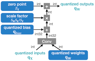
5.4.2 Convolution Layer

마찬가지로 convolution 연산 수식도 정리할 수 있다.

Y = C o n v (W, X) + b

$Z_{W} = 0$
$Z_{b} = 0$ , $S_{b} = S_{W} S_{X}$
$q_{b i a s} = q_{b} - C o n v (q_{w}, Z_{X})$

↓

q_{Y} = \frac{S_{W} S_{X}}{S_{Y}} (C o n v (q_{W}, q_{X}) + q_{b i a s}) + Z_{Y}

해당 수식의 연산 그래프는 다음과 같다.

linear quantization convolution graph

5.5 Hardware Implementation of Integer-Arithmetic-Only Inference

Quantization and Training of Neural Networks for Efficient Integer-Arithmetic-Only Inference 논문(2017)

tinyML Talks: A Practical Guide to Neural Network Quantization

다음은 uint8 양자화 모델을 추론하는 MAC array이다.

quantized MAC array

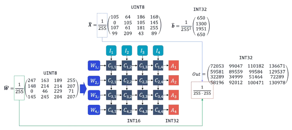
A_{i} = \sum_{j} C_{i, j} + b_{i}

5.6 Symmetric vs Asymmetric Quantization

unsigned int 타입의 양자화는 ReLU와 유사한 output activation을 대상으로 할 때 특히 유용하다.

	Symmetric (signed)	Symmetric (unsigned)	Asymmetric (unsigned)

Zero Point	$Z = 0$	$Z = 0$	$Z \neq 0$
INT8 Range	[-128, 127] (restricted) [-127,127] (full)	[0, 255]	[0, 255]
Matrix Transform	Scale	Scale	Affine

restricted range: full range 대비 정확도 떨어지지만, 연산 비용이 저렴하며 구현도 쉽다.

5.7 Sources of Quantization Error

linear quantization에서 양자화 오차를 발생시키는 원인을 알아보자.

$x \to x_{i n t}$

round error: $x$ 에서 근접한 값 $\to$ 동일한 $x_{i n t}$ grid
clip error: 범위( e.g., $q_{m a x}$ )를 벗어난 outlier $\to 2^{b} - 1$

quantization error = round error + clip error

다음은 양자화된 값 $x_{i n t}$ 을 $\hat{x}$ 로 복원한 뒤 발생한 오차를 나타낸 그림이다. scaling factor를 어떻게 정하는가에 따라, 양측 오차에서 trade-off가 발생한다.

$x_{i n t} \to \hat{x}$ (case 1: round error가 큰 경우)

$x_{i n t} \to \hat{x}$ (case 2: clip error가 큰 경우)

따라서, 양자화 시 최적의 절충점을 고려하여 scaling factor를 정해야 한다.