Lecture 04 - Pruning and Sparsity (Part II)
Lecture 04 - Pruning and Sparsity (Part II) | MIT 6.S965
EfficientML.ai Lecture 4 - Pruning and Sparsity (Part II) (MIT 6.5940, Fall 2023, Zoom recording)
weight 혹은 activation 값 중 하나가 0이면, 다음과 같이 곱 연산을 생략할 수 있다.
4.5 EIE: Parallelization on Sparsity
EIE: Efficient Inference Engine on Compressed Deep Neural Network 논문(2016)
EIE 논문은 weight sparsity 및 activation sparsity를 모두 활용하며, 다음과 같은 이점을 획득했다.
| weight sparsity (0 $\times$ A = 0) |
activation sparsity (W $\times$ 0 = 0) |
|
|---|---|---|
| 90% sparsity 기준 | 70% sparsity 기준 | |
| (+) | computation 10배 감소 memory footprint 5배 감소 |
computation 3배 감소 |
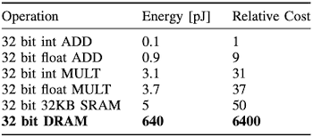
구체적으로는 sparsity를 활용하는 압축 알고리즘을 통해, DRAM memory access 비용을 절감했다.
45NM CMOS process 기준으로, SRAM에 비해 DRAM access가 128배나 되는 에너지를 소모한다.
4.5.1 Computation and Representation
다음 예시를 통해 EIE의 동작을 살펴보자.
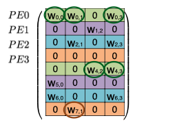
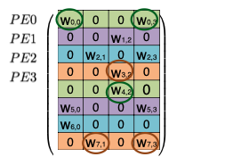
기본적으로 weight matrix $W$ 의 행을 interleaving하여 연산을 병렬화한다.
| Processing Element(PE) ( $N=4$ ) |
Sparse Matrix $\times$ Sparse Vector Operation ( Input Activation Vector $a$ $\times$ Weight Matrix $W$ ) |
|---|---|
 |
 |
동일한 PE에 저장되는 값은 동일한 색상으로 표기 (색상별로 하나의 큰 배열에 저장된다.)
(mod N) 연산을 통해 $N$ 개의 PE에 각각 대응되는 $W_i$ 를 분배한다.
모든 $PE$ 는 $W_i$ (weight row), $a_i$ (input activation) $b_i$ (output activation)를 보유하며, 가중치 행렬에서 non-zero 가중치만 벡터에 저장된다. 연산은 다음과 같은 순서로 진행된다.
| Step | Description |
|---|---|
| (i) | 입력에서 non-zero $a_j$ 를 찾은 뒤, PE에게 해당 index $j$ 를 broadcast한다. |
| (ii) | 각 PE는 $a_j$ 와 column $W_j$ 의 non-zero 값과 곱한 뒤, 결과를 output activation $b$ 에 누적한다.(MAC 연산) |
4.5.2 Compressing Sparse Matrix
EIE 논문은 CSC(Compressed Sparse Column) 포맷을 활용해 sparse weight matrix를 encoding한다. 먼저, 하나의 column을 encoding하는 예시를 살펴보자.
EIE처럼 $v, z$ entry는 4-bit 값(0~15)으로 양자화된다고 가정하며, 앞에 위치한 0의 개수가 15개를 넘어가는 부분에 주목하자. ( $v$ 는 이후 LUT를 참조하여, 16-bit fixed-point로 decoding된다.)
$$ [0,0,1,2,0,0,0,0,0,0,0,0,0,0,0,0,0,0,0,0,0,0,3] $$
| $v$ | non-zero 값을 담는 벡터 (Virtual Weight) |
$v = [1,2,\mathsf{0},3]$ |
| $z$ | $v$ 와 동일한 길이를 가지며, 각 $v$ entry마다 앞에 위치한 0의 개수(distance)를 담는다. (Relative Index) |
$z = [2,0,\mathsf{15},2]$ |
추가로 $v$ 와 $z$ 를 하나의 큰 배열 쌍에 저장하기 위해, 각 column의 첫 entry 위치를 가리키는 pointer vector $p$ 를 둔다. (Column Pointer)
column $j$ 에 위치한 모든 entry를 불러오려면, $p_j$ index부터 $(p_{j+1} -1)$ index까지 값을 모두 읽으면 된다.
다음은 sparse weight matrix에 CSC format encoding을 수행한 예시다.
| Logically | 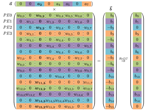 |
| Physically | 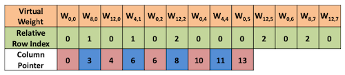 |
column $j$ #nonzero = $p_{j+1} - p_{j}$
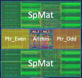
4.5.3 Micro Architecture for each PE
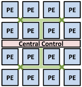
다음은 PE의 micro architecture를 나타낸 도식이다.
PE array를 제어하는
Central Control Unit(CCU)가, PE 내부의 큐로 non-zero activation을 broadcast한다. (queue가 가득차면 broadcast 중단)load imbalance에 의한 문제를 방지하기 위한 구현으로, PE는 큐에서 계속해서 activation을 읽어와 작업을 수행할 수 있다.(FIFO)
1 cycle에 2개 pointer를 모두 읽을 수 있도록, 두
Ptr SRAM Bank에서 각자 $p_j$ , $p_{j+1}$ 를 처리한다. (즉, $p_j$ , $p_{j+1}$ 는 항상 다른 bank에 위치한다.)
Sparse Matrix SRAM의 각 entry는 8 bit로 구성되며, 4-bit인 $v$ 와 $z$ 를 하나씩 포함한다.SRAM 자체의 width는 64-bit이므로 8개 entry를 한 번에 가져온다.
| Layout of PE | PE architecture |
|---|---|
 |
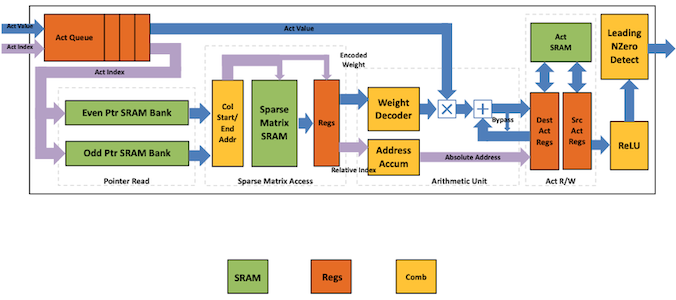 |
흐름을 단계별로 파악해 보자.
| 1. **Sparse Matrix Read Unit**   - 포인터 $p_j, p_{j+1}$ 를 활용해, (SRAM에서) column $j$ 의 nonzero 값을 읽어온다. - $(v, x)$ 를 전달한다. - $x$ : accumulator array index - $v$ : weight value > pointer $p$ (16 bits): 상위 13 bit는 SRAM row를 가리키고, 하위 3 bit는 entry(8개 원소) 중 하나를 가리킨다. |
| 2. **Arithmetic Unit**   - Sparse Matrix Read Unit에서 $(v, z)$ 값을 받아, MAC 연산( $b_{z} = b_{z} + v \times a_{j}$ )을 수행한다. > 이때, 4-bit로 사전에 양자화된 $v$ 를, LUT를 조회하여 16 bits로 decoding하는 과정을 거친다. |
| 3. **Write Back**  - 연산 결과를 SRAM에 저장한다. |
| 4. **ReLU**, **Non-zero Detection**  - ReLU 연산을 수행한다. > Leading Non-zero Detection Node(LNZD) 노드에서 nonzero activation를 찾아낸다.(다음 stage에서 활용) |
4.5.4 Benchmark of EIE
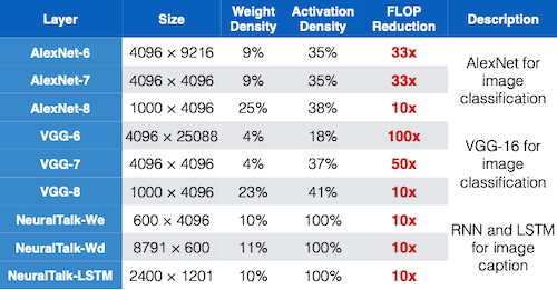
다음은 EIE를 활용해 다양한 모델을 추론한 결과이다.
- 특히, 0의 값을 갖는 weight나 activation 대상으로 연산을 생략하기 때문에, 극적인 연산량(FLOPs) 감소를 달성했다.
다음은 지연시간 및 에너지 관점에서, EIE와 다양한 하드웨어 추론 결과를 비교한 도표이다.
Intel Core i7-5930k CPU, NVIDIA TitanX GPU, NVIDIA Jetson TK1 Mobile GPU
| speedup | 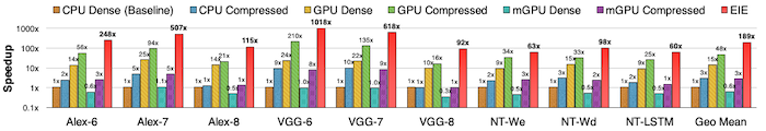 |
| energy | 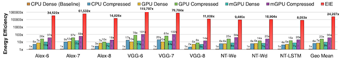 |
4.5.5 EIE: Pros and Cons
Retrospective: EIE: Efficient Inference Engine on Sparse and Compressed Neural Network 논문(2023)
위 논문에서는, EIE 접근법의 장단점을 다음과 같이 요약하고 있다.
| 장점 | 단점 |
|---|---|
| 연산량, 에너지 효율 fine-grained sparsity 지원 INT4까지 aggressive한 양자화 지원 |
control flow 관점에서 overhead, storage overhead structured sparsity 활용 불가 FC layers만 지원 SRAM에 주목한 최적화이므로, LLM 등 큰 모델에 비적합 |
4.6 ESE: Load Balance Aware Pruning
ESE: Efficient Speech Recognition Engine with Sparse LSTM on FPGA 논문(2016)
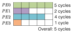
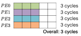
더 나아가 ESE 논문에서는, load balance를 고려하는 weight pruning 알고리즘을 제안했다.
- 모든 submatrix 단위에서 동일한 sparsity ratio를 갖도록 pruning한다.
| Unbalanced | Balanced |
|---|---|
 |
 |
 |
 |
(생략)