Lecture 04 - Pruning and Sparsity (Part II)
Lecture 04 - Pruning and Sparsity (Part II) | MIT 6.S965
EfficientML.ai Lecture 4 - Pruning and Sparsity (Part II) (MIT 6.5940, Fall 2023, Zoom recording)
4.1 Pruning Ratio
AMC: AutoML for Model Compression and Acceleration on Mobile Devices 논문(2018)
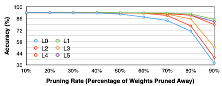
다음은 CIFAR-10으로 학습한 VGG-11 모델의 6개 레이어(L0\~L5)를 대상으로, pruning 시 정확도 변화(민감도)를 조사한 실험이다.(sensitivity analysis)
-
pruning ratio $r \in \lbrace 0, 0.1, 0.2, ..., 0.9 \rbrace$
-
정확도 감소( ${\triangle} {Acc}_{r}^{i}$ )가 제일 큰 레이어는 L0이다. 즉, L0 레이어가 제일 pruning에 민감하다.
단, 이러한 분석으로 얻은 pruning ratio는 최적이 아닌 한계를 갖는데, 이유는 레이어의 특징과 레이어 사이의 interaction이 고려되지 않기 때문이다.
예를 들어 레이어 크기가 작을 경우, pruning ratio가 커도 정확도 감소가 비교적 작다.
4.2 Finding Pruning Ratio: Learn to Prune
이후, 최적의 pruning ratio를 찾고자 하는 다양한 연구가 시도되었다.
4.2.1 Reinforcement Learning based Pruning: AMC
AMC: AutoML for Model Compression and Acceleration on Mobile Devices 논문(2018)
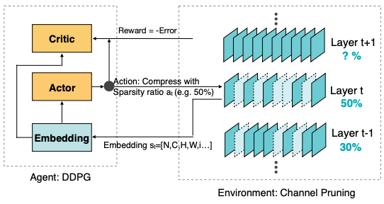
Agent(에이전트): Environment(환경)을 관찰하여 얻은 state(상태) 값 및 policy(정책)를 토대로 action(행동)을 결정한다.
때때로 행동에 대한 reward(보상)을 받는다.
policy: state를 입력으로 받아서, 출력으로 agent가 수행해야 하는 행동을 반환하는 함수
AMC(AutoML for Model Compression) 논문에서는, 최적의 pruning ratio를 Reinforcement Learning(강화 학습) 기반으로 탐색한다.
-
Agent: 레이어 $t$ 의 embedding state $s_t$ 를 입력으로, action인 sparsity ratio $a_t$ 를 출력한다.
-
embedding state $s_t = [N, C, H, W, i, ...]$
DDPG = Deep Deterministic Policy Gradient
- Reward: $-Error$ (error rate)로 정의된다.
이때, 제약조건(latency, FLOPs, model size 등)을 고려하는 패널티를 부여할 수 있다.
e.g., $R_{FLOPs} = -Error \cdot log(FLOPs)$
제약조건을 만족하지 않는 경우, Reward 값으로 $-\infty$ 를 준다.
$$ R = \begin{cases} -Error, & if \ \mathrm{satisfies} \ \mathrm{constraints} \ -\infty , & if \ \mathrm{not} \end{cases} $$
4.2.1.1 Sparsity Pattern Across Layers
다음은 ImageNet-1으로 학습한 ResNet-50에서 레이어별 획득한 density이다.
density = #non-zero_weights / #weights
이때, iterative pruning을 4 stage 동안 수행했다. (stage마다 전체 density를 각각 $[50\%,35\%,25\%,20\%]$ 으로 설정)
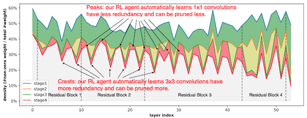
x축: layer index, y축: density. density 값이 클수록 sparsity ratio가 작다 = 더 민감하다.
| Peaks | 대부분 1x1 convolution(pointwise) | pruning에 민감하다. |
| Crests | 대부분 3x3 convolution(depthwise) | pruning에 덜 민감하며, 공격적인 가지치기가 가능하다. |
즉, 강화학습의 결과를 통해, 3x3 convolution을 더 가지치기하는 것이 효율적임을 알 수 있다.
4.2.1.2 Speedup Mobile Inference
ImageNet으로 학습한 MobileNet 대상으로 획득한 모델을 실제 추론하여 얻는 speedup 성능이다.
- Galaxy S7 Edge 추론에서, 25%의 pruning ratio로 1.7x speedup 획득
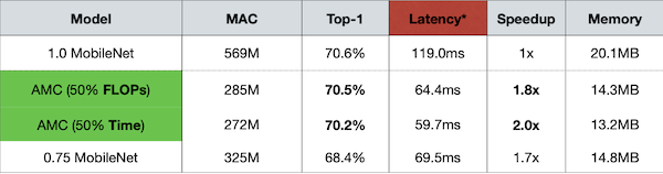
입력과 출력 모두 3/4씩 줄어드는 효과이므로, quadratic한 speedup을 획득하게 된다.
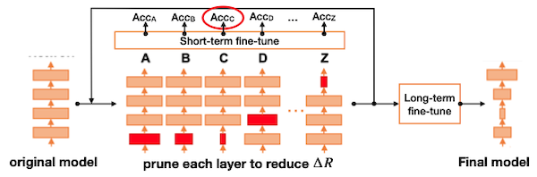
4.2.2 Rule based Pruning: NetAdapt
NetAdapt: Platform-Aware Neural Network Adaptation for Mobile Applications 논문(2018)
NetAdapt에서는 feedback loop 기반으로 최적의 pruning ratio를 탐색한다.
- 목표: 제약 조건(e.g., latency, energy, ...)을 만족하며 최고 정확도를 갖는 레이어별 pruning ratio
먼저 1 iteration마다 단일 레이어를 대상으로 pruning하며, 모델의 latency(제약조건)가 $\triangle R$ 만큼 줄어들 때까지 수행한다. (latency는 LUT를 통해 측정)
#pruned_models = #iterations
| original model | NetAdapt Iterative Pruning |
|---|---|
 |
 |
-
pruning 후, 짧게 10k iteration 동안만 fine-tuning하여 성능을 측정한다.
-
가장 높은 정확도를 갖는 모델은 다음 iteration의 초기 모델이 된다.
모든 iteration이 끝나면, 가장 높은 성능의 모델을 대상으로 long-term fine-tuning 후 성능을 측정한다.
4.2.3 Regularization based Pruning
Learning both Weights and Connections for Efficient Neural Networks 논문(2015)
Learning Efficient Convolutional Networks through Network Slimming 논문(2017)
A Systematic DNN Weight Pruning Framework using Alternating Direction Method of Multipliers(2018)
fine-tuning 및 training 과정에서, loss function에 regularization 항을 추가하여 sparsity를 향상시킬 수 있다.
- 가장 대표적으로 L1, L2 Regularization를 사용하는 weight pruning은, 다음과 같이 정의할 수 있다.
| Regularization | Loss Function |
|---|---|
| L1-Regularization | $L' = L(x; W) + \lambda |W|$ |
| L2-Regularization | $L' = L(x; W) + \lambda ||W||{}^2$ |
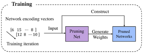
4.2.4 Meta-Learning based Pruning: MetaPruning
MetaPruning: Meta Learning for Automatic Neural Network Channel Pruning 논문(2019)
MetaPruning 논문에서는 최고 성능의 모델을 획득하기 위해, 가지치기된 구조를 입력으로 대응되는 가중치를 생성하는 meta network를 학습한다.
논문에서는 channel pruning 문제를, 제약조건을 만족하면서 loss가 최소화되는 channel width의 집합으로 정의한다.
$$ (c_1, c_2, \cdots, c_l)^{*} = \underset{c_1, c_2, \cdots, c_l}{\arg\min} \mathcal{L}(\mathcal{A}(c_1, c_2, \cdots, c_l ; w)) $$
$$ s.t. \quad C < \mathrm{constraint} $$
$c_l$ : $l$ 번째 레이어의 channel width, $C$ : cost(FLOPs, latency 등)
MetaPruning은 meta network인 PruningNet을 학습하는 단계와, PruningNet을 사용해 제약조건을 만족하며 최고 정확도를 갖는 모델의 탐색 단계로 구성된다.
| (Step 1) Training | (Step 2) Searching |
|---|---|
 |
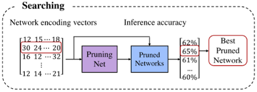 |
최적 모델의 탐색 알고리즘으로는 evolutionary search를 사용한다.
4.2.4.1 Meta Network: PruningNet
두 개의 fully-connected layer를 갖는 모델로 구성된 PruningNet은, 입력으로 encoding vector $(c_1, c_2, \cdots, c_l)$ 를 받아서, 출력으로는 생성한 pruned network의 가중치 $W$ 를 반환한다.
training iteration마다 무작위로 channel width 조합을 생성한다.
$$ W = \mathrm{PruningNet}(c_1, c_2, \cdots, c_l) $$
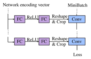
이후 pruned model은 Reshape 연산을 통해, PruningNet에서 입력으로 받은 $(c_1, c_2, \cdots, c_l)$ 와 동일한 출력 채널 수를 갖도록 구성된다.
- 해당 모델에 입력 이미지 배치를 통과시켜 loss를 계산하고, 연결된 PruningNet의 가중치를 업데이트한다.
4.3 Lottery Ticket Hypothesis
The Lottery Ticket Hypothesis: Finding Sparse, Trainable Neural Networks 논문(2019)
THE LOTTERY TICKET HYPOTHESIS: FINDING SPARSE, TRAINABLE NEURAL NETWORKS
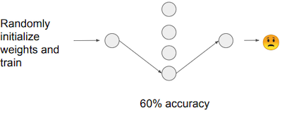
Lottery Ticket Hypothesis(LTH)는, 희소화된 네트워크를 from scratch( $W_{t=0}$ )부터 다시 학습했을 경우 갖는 성능에 의문을 제기한다.
- original pruned model: 90% accuracy 가정
| Pruned Model+From Scratch | Winning Ticket |
|---|---|
 |
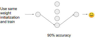 |
| 60% 정확도로, 전보다 낮은 성능 획득 | 90% 정확도로, 전보다 적은 학습만으로도 기존 이상의 성능 획득 |
즉, 기존 dense model보다 희소하면서, 적은 학습만으로도 기존 이상의 성능을 갖는 sub-network가 존재할 수 있다는 것이 LTH의 주장이다.
4.3.1 Iterative Magnitude Pruning
winning ticket을 찾는 가장 대표적인 방법으로, Iterative Magnitude Pruning이 존재한다.
성능 면에서 one-shot pruning 방법보다는, 여러 차례 과정을 반복하는 Iterative Pruning이 효과적이다.
다음은 iterative magnitude pruning 방법을 통해 winning ticket을 찾는 과정이다.
| Step 1 | dense model training $\rightarrow$ pruning $\rightarrow$ random initialization (same sparsity mask) |
 |
| Step 2 | training $\rightarrow$ pruning |  |
| Step 3 | random initialization (same sparsity mask) |
 |
| Step 4 | Repeat Step 2-3 |
이러한 Iterative Magnitude Pruning 방법에서는, 수렴까지 학습을 위한 비용이 소모된다는 단점에 주의해야 한다.
4.3.4 Limitation
하지만 한계점으로, (MNIST, CIFAR-10과 같은) 작은 데이터셋이 아니라 ImageNet과 같이 거대한 데이터셋에서는 정확도를 복구하지 못했다.

대안으로 특정 iteration까지 학습한 가중치( $W_{t=k}$ )를 활용하여, fine-tuning으로 정확도를 회복할 수 있다.
4.4 Pruning at Initialization(PaI)
보다 훈련 비용을 낮추기 위해, 훈련 전에 먼저 winning ticket을 찾는 Pruning at Initialization(PaI, a.k.a. Foresight Pruning) 방법이 제안되었다.
| Pruning after Training(PaT) |  |
| Pruning at Initialization(PaI) |  |
대체로 PaI는 PaT에 비해 성능이 떨어지기 때문에, 주로 효율적인 훈련(예: 훈련 속도)이 필요한 상황에서 활용된다.
4.4.1 SNIP: Connection Sensitivity
SNIP: Single-shot Network Pruning based on Connection Sensitivity 논문(2018)
최초로 PaI를 구현한 SNIP 논문은 가중치 연결을 on/off하며, loss에 얼마나 변화를 미치는지 관찰하고, 이를 기반으로 connection sensitivity를 계산한다.
- connection mask ( $c_j \in \lbrace 0, 1 \rbrace$ )를 도입하여 연결을 제어한다.
$c_j = 1$ (active), $c_j = 0$ (pruned)
- 예를 들어, connection $j \in \lbrace 1 \cdots m \rbrace$ 의 loss 변화는, 다음과 같이 계산할 수 있다.
$e_j$ : $j$ 번째 연결을 제외하고 모두 $0$ 값을 갖는 벡터
$$ \triangle L_j (w; \mathcal{D}) = L(1 \odot w; \mathcal{D}) - L((1 - e_j) \odot w; \mathcal{D}) $$
이때, Variance Scaling을 통해 가중치를 초기화하며, 입력으로는 훈련 데이터셋에서 샘플링한 하나의 minibatch를 활용한다.
다음은 SNIP에서 정의한 수식이다.
| Loss Function | Connection Sensitivity |
| $\min_{c,w} L(c \odot w; \mathcal{D}) = \min_{c,w} { {1} \over {n} } \sum\limits_{i=1}^n l(c \odot w ; (x_i, y_i))$ | $s_j = { {|g_{j}(w;\mathcal{D})|} \over { {\sum}^m_{k=1} |g_k(w;\mathcal{D})|} }$ |
| - $\mathcal{D}$ : training dataset - $\odot$ : Hadamard product | - $j \in \lbrace 1 \cdots m \rbrace$ - $e_j$ : $j$ 번째를 제외하고, 모두 0의 값을 갖는 vector |
이후 모든 connection sensitivity 계산이 끝나면, top- $\kappa$ 개 연결만을 남기고 일반적인 모델 학습 과정을 진행한다.
4.4.2 GraSP: Gradient Signal Preservation
PICKING WINNING TICKETS BEFORE TRAINING BY PRESERVING GRADIENT FLOW 논문(2020)
하지만 SNIP은 하나의 가중치 연결만 주목하면서, 가중치 사이의 복잡한 interaction은 포착하지 못한다. 또한, 중요한 연결을 제거하면서 모델에서 정보의 흐름이 차단될 수 있다.
SNIP에서는 높은 pruning ratio으로 설정 시, 특정한 레이어의 가중치를 모두 제거하는 문제가 발생한다.
이러한 SNIP의 단점을 해결하는 방안으로, GraSP 논문은 gradient flow의 관찰을 제안한다.
- (전제) 모델의 최종 성능은 trainability와 큰 연관이 있다.
$\rightarrow$ pruning 이후의 gradient flow를 관찰하여, 모델의 trainability를 파악할 수 있다.
다시 말해 pruning 이후의 기울기를 관찰하고, 이때 기울기의 크기(norm)이 크게 감소하면, 해당 연결이 중요한 연결이라고 판단할 수 있다.
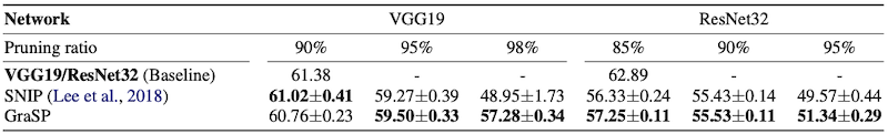
실제로 Tiny-ImageNet 대상으로 학습한 VGG19, ResNet32 실험에서, SNIP에 비해 높은 pruning ratio 설정에서 더 높은 정확도를 획득했다.