Lecture 03 - Pruning and Sparsity (Part 1)
Lecture 03 - Pruning and Sparsity (Part I) | MIT 6.S965
EfficientML.ai Lecture 3 - Pruning and Sparsity (Part I) (MIT 6.5940, Fall 2023, Zoom recording)
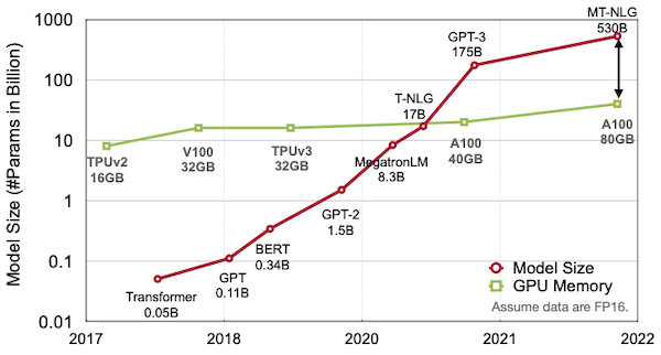
지금의 AI model size는 너무나 크다.
메모리 비용은 (연산 비용과 비교해서, 보다) expensive하다.
- register file access cost를 1로 뒀을 때, SRAM cache가 5배 cost, DRAM access가 약 640배 cost를 소비한다.
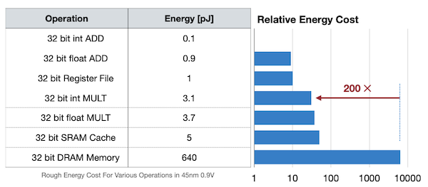
데이터 이동이 많을수록 memory reference가 필요하고, 이는 더 많은 power를 필요로 하게 된다. 그렇다면 이러한 비용을 어떻게 줄일 수 있을까? 대표적으로는 다음과 같은 방법들을 고려할 수 있다.
-
model/activation size 줄이기
-
workload 줄이기(data를 빠르게 compute resources에 공급)
-
compiler/scheduler 개선하기
-
locality를 활용하기
-
cache에 더 많은 data를 보관하기
이중에서도 모델의 over-parameterization에 의한 비용을 해결하기 위한 효과적인 방법인 pruning(가지치기)을 살펴볼 것이다.
pruning은 1990년부터 제시된 역사가 깊은 기법이다. 1993년에는 pruning 이후 weight를 fine-tuning하는 방법을 제시했다.
3.1 Pruning
prining은 크게 세 가지 단계로 구성된다.
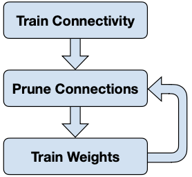
- Train Connectivity
over-parameterized target network를 학습한다.
- Prune Connections
weight(unit) importance를 파악 후, 중요하지 않은 weight를 pruning한다.
- Train Weights
pruning 이후의 정확도 손실을 fine-tuning으로 보완한다.
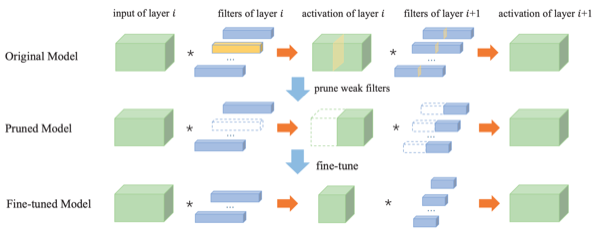
3.1.1 Pruning and Fine-tuning
Learning both Weights and Connections for Efficient Neural Networks 논문(2015)
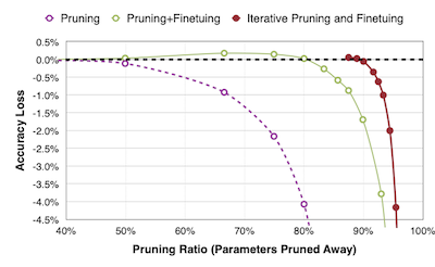
다음은 AlexNet에 세 가지 다른 방법으로 pruning했을 때, 정확도 손실을 나타낸 그래프이다.
-
Pruning
-
50%: 비교적 정확도 손실이 적다.
-
80%: 4%가 넘는 정확도 손실이 발생한다.
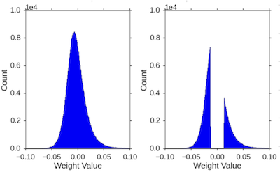
정규 분포를 이루던 가중치 분포는, pruning을 거치면 다음과 같이 변화한다.
-
-
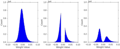
Pruning + Fine-tuning
80%를 pruning 후, 남은 20%의 가중치를 fine-tuning한다. fine-tuning 후 가중치 분포는 다음과 같이 smooth하게 변화한다.
-
Iterative Pruning + Fine-tuning
2번 과정을 반복하면, 매우 적은 정확도 손실로 약 90% 수준까지 가중치 pruning이 가능하다.
3.1.2 CNN + Pruning Results
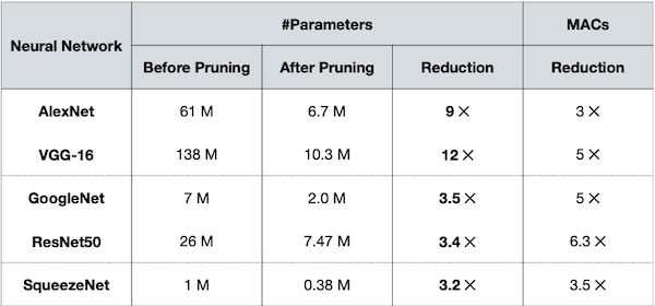
다음은 여러 network에 pruning을 적용하고 난 뒤 결과를 정리한 표다.
-
AlexNet, VGG-16는 pruning을 통해 9배, 12배가 넘게 크기를 줄였다.
-
반면, GoogleNet, ResNet, SqueezeNet과 같은 compressed model에서는 큰 효과를 보지 못했다.
이런 경우 quantization(양자화) 같은 수단이 더 효과적이다.
3.1.3 MLPerf Inference
Leading MLPerf Inference v3.1 Results with NVIDIA GH200 Grace Hopper Superchip Debut
MLPerf는 다양한 기업이 참가하는 Al computing 대회다. closed division과 open division 두 트랙에서 경쟁한다.
- closed division
신경망을 변경할 수 없다.(precision, weight 등) 따라서 오로지 hardware innovation으로 경쟁해야 한다.
- open division
신경망을 변경할 수 있다. 모델을 수정 혹은 압축하는 등 다양한 기법으로 경쟁한다.
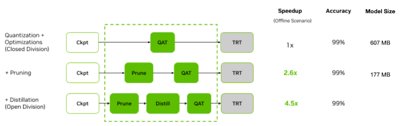
핵심은 두 트랙 모두 정확도를 잃지 않으면서, 빠르게 추론해야 한다. 아래는 BERT를 대상으로 한 NVIDIA의 closed, open division 결과물이다.
| closed division | open division | speedup | |
|---|---|---|---|
| offline samples/sec | 1029 | 4609 | 4.5x |
open division에서 4.5x 더 빠르게 sample 처리
이때 다음 기법으로 4.5x의 speedup을 획득했다.
-
Pruning
-
Quantization-Aware Training(QAT)
-
Knowledge Distillation
3.1.4 Pruning in the Industry
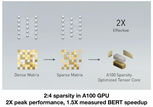
대표적으로 NVIDIA는 hardware 수준의 sparsity matrix을 이용한 가속을 지원하고 있다. 특정 조건을 만족하면 dense matrix를 sparse matrix로 바꿔서 연산을 가속할 수 있다.
-
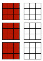
2:4 sparsity: 4개의 parameter로 이루어진 그룹에서 paramter 2개가 0이면 가능하다.
3.2 Formulate Pruning
일반적으로 Pruning은 손실 함수에서, #non-zero 수의 threshold $N$ 을 두어 제한하는 것으로 구현할 수 있다.
$$ \underset{W_p}{\mathrm{argmin} }{L(\mathbf{x}; W_p)} $$
$$ s.t. {||W_{p}||}_{0} \le N $$
-
$W_{p}$ : pruned weights
-
$N$ : threshold
s.t.: subject to
L0-norm: = #nonzeros
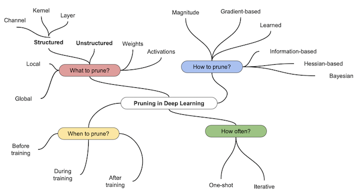
3.3 What, How, When, How often to prune
pruning은 어떤 단위로, 어떤 기준으로, 언제, 얼마나 자주 적용해야 하는가에 따라 세부적으로 나눌 수 있다.
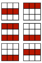
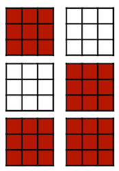
3.4 Pruning Granularity
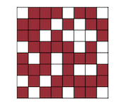
pruning을 적용하는 granularity는, 크게 unstructured, structured pruning으로 나눌 수 있다.
| Unstructured (weight-wise) |
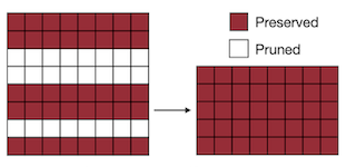
Structured (Channel, Kernel, Layer, ...) |
|
|---|---|---|
 |
 |
|
| compression ratio | 크다 | 작다 |
| acceleration | 어렵다 | 비교적 쉽다 |
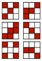
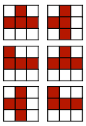
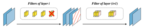
3.4.1 Pruning at Different Granularities
보다 세부적으로 pruning granularity를 살펴보자.
| Fine-grained | Pattern-based | Vector-level | Kernel-level | Channel-level |
|---|---|---|---|---|
 |
 |
 |
 |
 |
좌측에 위치할수록 fine-grained, 우측에 위치할수록 coarse-grained
3.4.2 Pattern-based Pruning: N:M sparsity
(생략)
3.4.3 Channel Pruning
이때 채널별로 최적의 pruning ratio를 탐색하면, 더 좋은 성능을 얻을 수 있다.
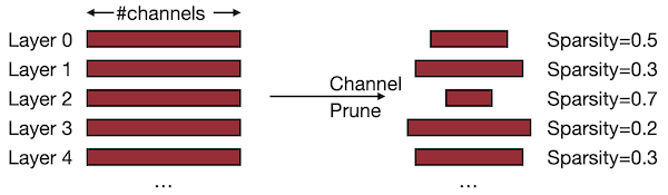
-
(+) direct하게 speedup을 구현할 수 있다.
-
(-) compression ratio이 낮다.
-
(-) 출력에 영향을 미치는 것을 주의해야 한다.(특히 residual connection 사용 시)
3.5 Pruning Criterion
pruning은 기본적으로 덜 중요한 파라미터를 제거하는 과정이다.
3.5.1 Magnitude-based Pruning: L1-norm
Learning both Weights and Connections for Efficient Neural Networks 논문(2015)
heuristic에 기반하여, 파라미터의 절댓값 크기를 importance로 사용할 수 있다.(L1-norm)
$$ Importance = \sum_{i \in S}|w_i| $$
다음은 예시 행렬에서 중요도 50%를 충족하는 파라미터만 남긴 결과다.
$$ \begin{bmatrix} 3 & -2 \ 1 & -5 \end{bmatrix} $$
- Element-wise
$$ \begin{bmatrix} |3| & |-2| \ |1| & |-5| \end{bmatrix} \rightarrow \begin{bmatrix} 3 & 0 \ 0 & -5 \end{bmatrix} $$
- Row-wise
$$ \begin{bmatrix} |3| + |-2| \ |1| + |-5| \end{bmatrix} \rightarrow \begin{bmatrix} 0 & 0 \ 1 & -5 \end{bmatrix} $$
3.5.2 Magnitude-based Pruning: L2-norm
혹은 L2-norm이나, $L_p$ norm을 사용할 수도 있다.
$$ Importance = \sqrt{\sum_{i \in S}{ {|w_{i}|}^{2} } } $$
다음은 예시 행렬을 대상으로 적용한 결과다.
$$ \begin{bmatrix} 3 & -2 \ 1 & -5 \end{bmatrix} $$
- Element-wise
$$ \begin{bmatrix} \sqrt{|3|^2} & \sqrt{|-2|^2} \ \sqrt{|1|^2} & \sqrt{|-5|^2} \end{bmatrix} \rightarrow \begin{bmatrix} 3 & 0 \ 0 & -5 \end{bmatrix} $$
- Row-wise
$$ \begin{bmatrix} \sqrt{|3|^2 + |-2|^2} \ \sqrt{|1|^2 + |-5|^2} \end{bmatrix} \rightarrow \begin{bmatrix} 0 & 0 \ 1 & -5 \end{bmatrix} $$
3.5.3 Sensitivity and Saliency
SNIP: Single-shot Network Pruning based on Connection Sensitivity 논문(2018)
SNIP 논문에서는 connection sensitivity라는 salience 기반의 pruning criterion을 제시했다. 제거했을 때 sensitivity가 클수록 중요한 가중치로 고려한다.
$$ s_j(w; \mathcal{D}) = { {|g_{j}(w;\mathcal{D})|} \over { { {\sum}^m_{k=1} } |g_k(w;\mathcal{D})|} } $$
-
$s_j$ : weight $w_j$ 의 sensitivity
-
$m$ : #weights
-
$c_j$ : connection(active = 1, pruned = 0)
-
$g_j$ : $c_j$ 에 대한 loss $L(c \odot w)$ 의 미분
3.5.4 Loss Change: First-Order Taylor Expansion
weight saliency를 pruning 이후 손실 변화로 정의한다. 대표적으로 1차 테일러 근사를 활용하면, weight에 작은 변화(perturbation)가 생겼을 때의 변화를 측정할 수 있다.
$$ \triangle \mathcal{L} = \mathcal{L} (w + \triangle w) - \mathcal{L}(w) = {\nabla}_w \mathcal{L} \triangle w $$
- $\triangle w$ : weight perturbation
예를 들어 Gate Decorator 논문에서는, Batch Normalization에서 학습 가능한 scaling factor $\phi$ 를 추가하는 GBN(Gate Batch Normalization) pruning을 제안하였다.
$$ \hat{z} = \phi z $$
$z$ : 필터 $k$ 의 feature map. ( $\phi$ 를 0으로 만들면 해당 채널(필터)는 제거된다.)
$$ \triangle \mathcal{L_{\Omega}} (\phi) = | \mathcal{L_{\Omega}} (\phi) - \mathcal{L_{\Omega}} (0) | $$
-
테일러 전개를 통해, $\phi$ 를 0으로 만들었을 때의 손실 $\mathcal{L}$ 변화를 측정한다.
-
중요도가 낮은 필터 일부를 제거 후 미세조정한다. (이때 $\phi$ 에 sparse constraint를 두어 0에 가까운 필터가 발생하게 된다.)
Notes: shortcut connection 합산 시 채널 크기가 불일치할 문제를 고려해, 그룹 단위로 필터를 제거한다.
3.5.5 Loss Change: Second-Order Taylor Expansion
Group fisher pruning for practical network compression 논문(2021)
굉장히 오래 전부터 사용된 방법으로, 손실 함수의 2차 테일러 근사를 바탕으로 중요도를 계산한다.
$$ \mathcal{L} (w + \triangle w) - \mathcal{L}(w) = {\nabla}_w \mathcal{L} \triangle w + { {1} \over {2} } {\triangle}w^{T}H \triangle w $$
-
$H = {\triangle}_w^2 \mathcal{L}(w)$
-
신경망이 수렴한다고 가정하면, first-order 항은 0에 가까운 값으로 무시할 수 있다.
-
단점: Hessian matrix 계산 비용
3.6 Data-Aware Pruning Criterion
가중치만으로 최적의 가지치기 성능을 탐색하는 것은 어렵다. 따라서, 입출력을 활용한 data-aware pruning 방법이 등장했다.
3.6.1 Average-Percentage-Of-Zero-based Pruning(APoZ)
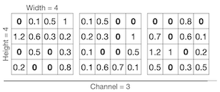
Network Trimming 논문에서는 출력 값에서 0을 갖는 비율을 바탕으로 한 pruning 방법을 제안하였다. 예를 들어 다음과 같은 output activations이 있다고 하자.
| Batch 1 | Batch 2 |
|---|---|
 |
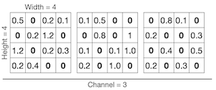 |
이때 각 배치마다 같은 위치에 있는 채널마다 0의 비율을 계산한다. (Average Percentage of Zeros(APoZ))
-
channel 0
-
batch 1 #zeros: 5
-
batch 2 channel 0 #zeros: 6
$$ { {5+6} \over {2 \cdot 4 \cdot 4} } = {11 \over 32} $$
-
channel 1
-
batch 1 #zeros: 5
-
batch 2 #zeros: 7
$$ { {5+7} \over {2 \cdot 4 \cdot 4} } = {12 \over 32} $$
-
channel 2
-
batch 1 #zeros: 6
-
batch 2 #zeros: 8
$$ { {6+8} \over {2 \cdot 4 \cdot 4} } = {14 \over 32} $$
예시에서는 0의 비율이 가장 많은 channel 2를 제거한다.
3.6.2 Regression-based Pruning: Reconstruction Error
Channel Pruning for Accelerating Very Deep Neural Networks 논문(2017)
위 논문에서는 feature map이 갖는 redundancy에 주목하여, 채널 제거 후 다음 레이어로 전달되는 출력 값이 이전과 동일하게 유지하는 데 집중한다.
-
$\beta$ : 채널 선택을 위한 마스크 계수 (LASSO 회귀, 즉 L1 정규화를 통해 도출)
-
$\beta_i$ 가 0이 되면 채널을 제거한다.
| Before Pruning ( 출력 $Z$ ) | After Pruning ( 출력 $\hat{Z}$ ) |
|---|---|
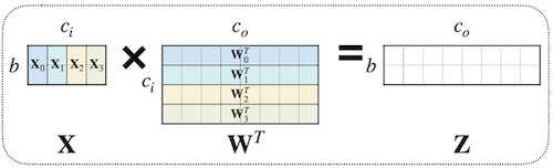 |
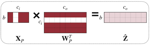 |
output activation $\hat{Z}$ 와 $Z$ 의 차이를 최소화하는 손실 함수는 다음과 같다.
$$ {\mathrm{arg} }\underset{W, {\beta} }{\mathrm{min} }{||Z-\hat{Z}||}^{2}{F} = || Z - \sum}^{c_{i}-1}{||{ {\beta{c}X $$}{W_{c} }^{T} }||}^{2}_{F
$$ s.t. \quad {||\beta||}{0} \le N $$
$N_{c}$ : #nonzero channels
3.6.3 Entropy-based Pruning
An entropy-based pruning method for cnn compression 논문(2017)
정보 이론(information theory) 관점에서 entropy가 크면 정보량이 많다는 것을 의미한다. 위 논문에서는 entropy가 높은 top $k$ 필터만 보존하는 pruning을 제안하였다.
필터가 만약 0 혹은 이와 유사한 값만 출력할 경우, 해당 채널은 entropy가 낮다고 판단한다.
각 필터에 대한 entropy 계산은 다음 절차로 이루어진다.
(1) output activation에 GAP(Global Average Pooling) 적용하여 1차원 벡터 획득
(2) 여러 학습 데이터에서 (1)을 수집하여 행렬 구성
(3) 각 채널별 값의 분포를 $m$ 개의 구간(bin)으로 나누고, 값이 각 구간에 속할 확률 $p_i$ 계산
(4) 각 채널의 entropy를 계산한다.
$$ H_j = -\sum_{i=1}^{m} p_i \log p_i $$
APoZ와 대비해, '0에 매우 가깝지만 0이 아닌 값을 주로 갖는 필터'를 제거하는 데 효율적이다.