Lecture 02 - Basics of Neural Networks

Lecture 02 - Basics of Neural Networks | MIT 6.S965

2.5 Efficiency Metrics

보통 network를 설계할 때, 크게 세 가지 요소를 고려한다.

• latency

• storage

• energy

그렇다면 다른 network 사이에서 efficiency(효율성)을 비교할 때 어떤 지표를 사용하여 비교해야 할까?

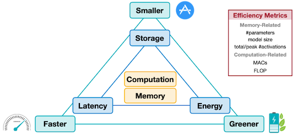
storage가 weight만 의미한다면, memory는 추가로 activation까지 고려한다.

• Memory-Related

• #parameters

• model size

• total/peak #activations

• computation

• MACs

• FLOP

2.5.1 Latency

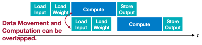
Neural Network 추론에 있어서, latency(지연시간)는 NN 자체의 특성과 hardware 특성에 모두 영향을 받는다. 예를 들어 pipelining을 이용하면 computation과 data movement는 동시에 이루어질 수 있다.

병렬화가 가능한 자원만 충분하다면 latency는 다음 수식으로 계산할 수 있다.

$$ Latency \approx \max(T_{computation}, T_{memory}) $$

• $T_{computation}$

분모는 hardware 특성, 분자는 NN 특성이다.

$$ \approx { {Number \ of \ Operations \ of \ NN} \over {Number \ of \ Opeartions \ that \ Processor \ can \ Process \ Per \ Second} } $$

• $T_{memory}$

$$ \approx T_{data \ movement \ of \ activations} + T_{data \ movement \ of \ weights} $$

• $T_{data \ movement \ of \ weights}$

분모는 hardware 특성, 분자는 NN 특성이다.

weight를 SRAM에 모두 저장하면, main memory에 접근하지 않을 수 있다.

$$ \approx { {Model \ size} \over {Memory \ Bandwidth \ of \ Processor} } $$

• $T_{data \ movement \ of \ activations}$

$$ \approx { {Input \ activation \ size + Output \ activation \ size} \over {Memory \ Bandwidth \ of \ Processor} } $$

2.5.2 Energy Consumption

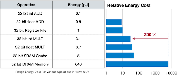
(생략)

2.5.3 Number of Parameters (#Parameters)

#Parameters는 기본적으로 총 weight 개수를 의미한다. 여러 레이어 종류에 따른 #Parameters를 구해보자.(bias는 무시)

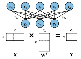
• Linear Layer

$W^{T}$ : 입력 채널 수( $c_i$ )와 출력 채널 수( $c_o$ )를 곱하면 된다.

$$ c_o \cdot c_i $$

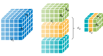
• Convolution

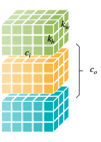
$$ c_o \cdot c_i \cdot k_h \cdot k_w $$

• Grouped Convolution

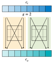
$$ c_o/g \cdot c_i/g \cdot k_h \cdot k_w \cdot g $$

$$ = c_o \cdot c_i \cdot k_h \cdot k_w / g $$

• Depthwise Convolution

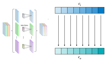
$$ = c_o \cdot k_h \cdot k_w $$

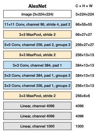
   📝 예제 1: AlexNet #Parameters    

AlexNet의 #Parameters를 구하라. 단, bias는 무시한다.

   🔍 풀이   

레이어별 #parameters를 구해보자.

• Conv Layer 1

$$ 96 \times 3 \times 11 \times 11 = 24,848 $$

• Conv Layer 2(grouped convolution 1)

$$ { {256 \times 96 \times 5 \times 5} \over {2} } = 307,200 $$

• Conv Layer 3

$$ 384 \times 256 \times 3 \times 3 = 884,736 $$

• Conv Layer 4(grouped convolution 2)

$$ 384 \times 384 \times 3 \times 3 / 2 = 663,552 $$

• Conv Layer 5(grouped convolution 3)

$$ 256 \times 384 \times 3 \times 3 / 2 = 442,368 $$

• Linear Layer 1

$$ 4096 \times (256 \times 6 \times 6) = 37,738,736 $$

• Linear Layer 2

$$ 4096 \times 4096 = 16,777,216 $$

• Linear Layer 3

$$ 1000 \times 4096 = 4,096,000 $$

모든 레이어의 #parameters를 합치면 총 61M이다.

2.5.4 Model Size

model size는 weight가 동일한 bit width를 가진다면 간단히 구할 수 있다.

bit width가 다른 mixed precision model은 계산이 달라진다.

• Model Size = #Parameters $\cdot$ Bit Width

   📝 예제 2: AlexNet model size    

AlexNet이 #Parameters를 61M만큼 갖는다고 할 때, 각 조건에서의 model size를 구하라.

• weight: fp32 type

• weight: int8 type

   🔍 풀이   

• fp32 type(=4 bytes)

$$ 61M \times 4Byte = 224MB $$

• int8 type(=1 byte)

$$ 61M \times 1Byte = 61MB $$

$1MB = 1 \times 10^6 Bytes$

2.5.5 Number of Activations (#Activations)

ResNet과 MobileNetV2를 비교해 보자.

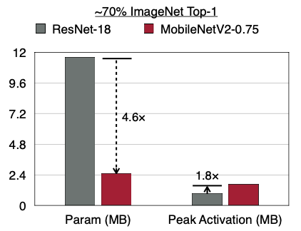
• MobileNetV2: ResNet보다 #Parameter는 적지만, 반대로 Peak Activation은 늘었다.

이는 MobileNetV2의 특정 레이어에서 #activations이 memory bottleneck을 일으키는 구조이기 때문이다.

MCUNetV2: Memory-Efficient Patch-based Inference for Tiny Deep Learning 논문

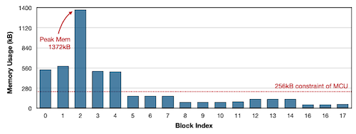
• 입력부와 가까운 레이어의 activation memory가 굉장히 크다.

• 반대로 resolution가 줄어들며 channel 수가 많아지는 후반부는 activation memory가 줄어들지만, 그만큼 많은 filter를 사용하므로 weight memory가 굉장히 커진다.

또한 훈련 중에도 memory bottleneck의 주된 원인은 #Parameter가 아닌 #activations이다.

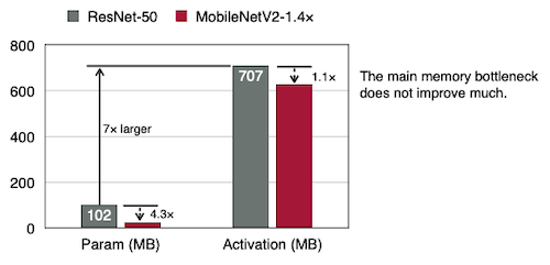
• #Parameter, #activations: FP32

• MobileNetV2이 ResNet보다 #Parameter가 4배 더 적지만, #activations은 1.1배 적다.

   📝 예제 3: AlexNet #Activations    

AlexNet의 (1) Total #Activations, (2) Peak #Activations를 구하라.

   🔍 풀이   

$$ 3 \times 224 \times 224 = 150,528 $$

$$ 96 \times 55 \times 55 = 290,400 $$

$$ 96 \times 27 \times 27 = 69,984 $$

...

$$ 256 \times 6 \times 6 = 9,216 $$

$$ 4096 = 4096 $$

$$ 4096 = 4096 $$

$$ 1000 = 1000 $$

따라서 Total #Activations, Peak #Activations은 다음과 같다.

• Total #Activations

$$ = 932,264 $$

• Peak #Activations

$$\approx input \ activations + output \ activations $$

$$= 150,528 + 290,400 = 440,928$$

2.5.6 MACs

computation efficiency를 표현하는 대표적인 지표인 MAC(Multiply-Accumulate) operations를 살펴보자.(MAC 연산은 CNN 연산의 대부분을 차지한다.)

우선 Multiply-Accumulate operation(MAC)은 다음과 같이 곱셈과 덧셈으로 이루어진 연산을 의미한다.

$$ a \leftarrow a + b \cdot c $$

두 가지 대표적인 연산에서 MACs를 구해보자.

• Matrix-Vector Multiplication(MV)

Matrix-Vector Multiplication 연산에서 MACs는 다음과 같이 계산할 수 있다.

![Matrix-Vector](https://raw.githubusercontent.com/erectbranch/MIT-Efficient-AI/master/2022/lec02/summary02/images/Matrix-Vector.png)

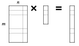
$$ MACs = m \cdot n $$

• General Matrix-Matrix Multiplication(GEMM)

Matrix-Matrix 연산에서 MACs는 다음과 같이 계산할 수 있다.

![General Matrix-Matrix](https://raw.githubusercontent.com/erectbranch/MIT-Efficient-AI/master/2022/lec02/summary02/images/General_Matrix-Matrix.png)

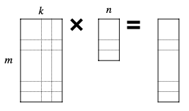
$$ MACs = m \cdot n \cdot k $$

이번에는 여러 레이어 종류별로 계산해 보자.(batch size n=1로 가정)

• Linear Layer

$$ MACs = c_o \cdot c_i $$

• Convolution

$$ MACs = c_i \cdot k_h \cdot k_w \cdot c_o \cdot w_o \cdot c_o $$

$w_o, c_o$ 계산에 주의.

다시 말해 output activation 각 픽셀마다 $c_i \cdot k_h \cdot k_w \cdot c_o$ 만큼의 MACs를 갖는다는 뜻이기도 하다.

• Grouped Convolution

$$ MACs = c_i/g \cdot k_h \cdot k_w \cdot c_o \cdot w_o \cdot c_o $$

• Depthwise Convolution

$$ MACs = k_h \cdot k_w \cdot c_o \cdot w_o \cdot c_o $$

   📝 예제 4: AlexNet #MACs    

AlexNet의 #MACs를 구하라.

   🔍 풀이   

• Conv Layer 1

$$ 96 \times 3 \times 11 \times 11 \times 55 \times 55 = 105,415,200 $$

• Conv Layer 2

$$ 256 \times 96 \times 5 \times 5 \times 27 \times 27 / 2 = 223,948,800 $$

...

• Linear Layer 1

$$ 4096 \times (256 \times 6 \times 6) = 37,748,736 $$

• Linear Layer 2

$$ 4096 \times 4096 = 16,777,216 $$

• Linear Layer 3

$$ 1000 \times 4096 = 4,096,000 $$

따라서 총 MACs는 724M이다.

2.5.7 FLOP

MAC과 마찬가지로 computation과 관련된 대표적인 지표로 FLOP(Floating Point Operations)이 있다.

processor의 성능 지표인 FLOPS(Floating Point Operation Per Second)와 구분할 것

만약 operations이 다음과 같은 data type이라면, 1 MAC = 2 FLOP이다.

• multiply: FP32

• add: FP32

   📝 예제 5: AlexNet #FLOP    

AlexNet의 FLOPs를 구하라. AlexNet은 총 MACs를 724M개를 갖는다고 한다.

• multiply: FP32

• add: FP32

   🔍 풀이   

$$ 724M \times 2 = 1.4G $$