Lecture 02 - Basics of Neural Networks
Lecture 02 - Basics of Neural Networks | MIT 6.S965
Lecture 5 slide: Image Classification with CNNs | Stanford CS231n
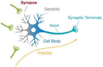
| 실제 뉴런과 시냅스 | 신경망(Neural Network) |
|---|---|
 |
 |
-
synapse: axon(축삭)과 dendrite(수상돌기)를 연결하여, 두 신경세포 사이의 연결을 담당한다.
-
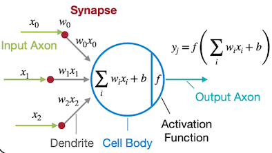
신경망 synapse
-
입력: 여러 input axon.
-
출력: 가중치를 곱하여 결합한 뒤 activation function(활성 함수)를 적용한 값을 반환한다.
2.1 Terminology of Fully-Connected Layer
다음은 3개 레이어(2개의 hidden layer)로 구성된 Fully-Connected Layer 예시이다.
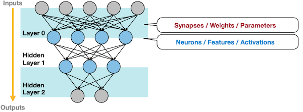
| 용어 | 신경망에서의 대응(동의어) |
|---|---|
| Synapse | parameter, weight |
| Cell body | sum of weighted inputs + bias |
| Neuron | feature, activation |
2.2 Shape of Tensors
$n$ : batch size, $c$ : channels, $w$ : width, $k$ : kernel size
2.2.1 Fully-Connected Layer
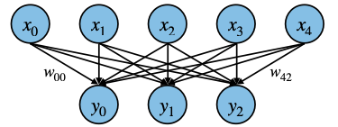
$$ y_i = \sum_{j}w_{ij}x_{j} + b_{i} $$
fully-connected layer의 tensor shape은 다음과 같다.
| Tensors | |
|---|---|
| Input Features $X$ | $(n, c_i)$ |
| Output Features $Y$ | $(n, c_o)$ |
| Weights $W$ | $(c_o, c_i)$ |
| Bias $b$ | $(c_o, )$ |
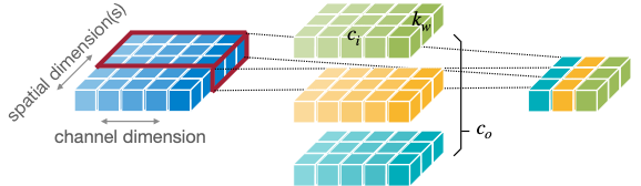
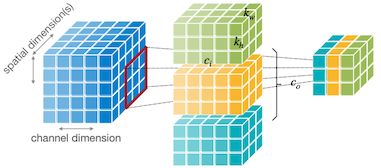
2.2.2 Convolution Layer
A guide to convolution arithmetic for deep learning 논문
그림의 텐서는 순서대로 입력, 필터, 출력 텐서에 대응된다.
다음은 1차원 및 2차원 Convolution Layer(합성곱 레이어)의 예시이다.
| Tensors | 1D Convolution | 2D Convolution |
|---|---|---|
 |
 |
|
| Input Features $X$ | $(n, c_i, w_i)$ | $(n, c_i, h_i, w_i)$ |
| Output Features $Y$ | $(n, c_o, w_o)$ | $(n, c_o, h_o, w_o)$ |
| Weights $W$ | $(c_o, c_i, k_w)$ | $(c_o, c_i, k_h, k_w)$ |
| Bias $b$ | $(c_o, )$ | $(c_o, )$ |
이때 합성곱 레이어는 하나의 필터(=kernel)가 하나의 출력 채널을 만들며, 필터를 shift하면서 여러 번 연산하는 방식으로 출력을 산출한다. (weight sharing)
출력 채널의 수 = 필터의 수
출력 텐서의 height $h_o$ 는 다음과 같이 계산할 수 있다.
$$ h_o = h_i - k_h + 1 $$
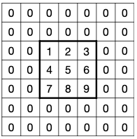
2.2.3 Convolution Layer: Padding
PyTorch의 default padding은 zero padding.
서로 다른 레이어에서 출력 텐서의 크기를 조절하기 위해 padding을 사용할 수 있다. (예를 들어, 입력 텐서와 동일한 resolution을 출력 텐서에서 유지) 다음은 세 가지 대표적인 padding 방법이다.
| Zero Padding | Reflection Padding | Replication Padding |
|---|---|---|
 |
 |
 |
출력 텐서의 height $h_o$ 는 다음과 같이 계산할 수 있다. ( $p$ : padding size )
$$ h_o = h_i + 2p - k_h + 1 $$
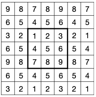
2.2.4 Convolution Layer: Receptive Field
합성곱 연산에서는 출력의 픽셀은 입력의 넓은 픽셀(higher level features)에 대응된다. 이를 수치화한 개념을 receptive field라고 한다.
- 각 output element: input에서 $k_{h} \times k_{w}$ receptive field를 가진다.
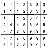
3개의 레이어를 거칠 때 receptive field가 어떻게 변화하는지 살펴보자.
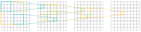
-
레이어를 거칠수록 $k-1$ 만큼 receptive field size가 커진다. ( $k=3$ 일 경우 1, 3, 5, 7, ...)
-
따라서, receptive field size는 다음과 같이 계산할 수 있다.
$$ L \cdot (k-1) + 1 $$
예시 그림에서 $L=3, k=3$ 이므로, receptive field size는 $3 \cdot (3-1) + 1 = 7$ 이다.
이러한 특성 때문에, CNN은 downsampling을 통해 해상도가 점차 줄어드는 것이 일반적이다. (downsampling이 없을 경우, 매우 많은 수의 레이어가 필요하므로)
$L=2, k=3$ 일 경우, receptive field size는 $2 \cdot (3-1) + 1 = 5$ 이다.
2.2.5 Strided Convolution Layer
receptive field가 더 넓어지기 위한 방법으로, 합성곱 연산에서 큰 stride 크기를 사용할 수 있다. 이를 strided convolution이라고 한다. 예를 들어 stride가 2일 경우, 필터는 한 번에 2칸씩 shift한다.
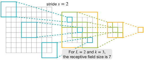
stride를 고려할 경우, receptive field size는 다음 수식으로 계산할 수 있다.
$$ \sum_{i=1}^{L}((k_i-1) \cdot \prod_{j=1}^{l-1} s_j) + 1 $$
$L=2, k=3$ 이며, 첫 번째 연산에서 stride $s=2$ 일 때, receptive field size는 다음과 같다.
$$ (3-1) \cdot 2 + (3-1) \cdot 1 + 1 = 7 $$
출력 텐서의 height $h_o$ 는 다음과 같이 계산할 수 있다. ( $p$ : padding size, $s$ : stride )
$$ h_o = \frac{h_i + 2p - k_h}{s} + 1 $$
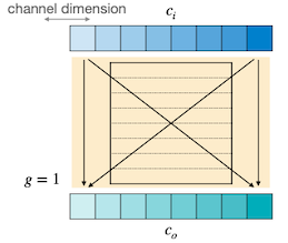
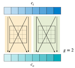
2.2.6 Grouped Convolution Layer
CNN에서 가중치의 수를 줄이기 위한 방법(=narrow하게 만들기 위한) 중 하나인 grouped convolution에서는, 입력 채널을 여러 그룹으로 나누고 각 그룹에서 별도의 필터로 연산한다. (따라서 그룹별로 병렬 연산도 가능하다.)
| convolution ( $g=1$ ) | grouped convolution ( $g=2$ ) |
|---|---|
 |
 |
grouped convolution의 tensor shape은 다음과 같다.
| Tensors | Grouped Convolution |
|---|---|
| Input Features $X$ | $(n, c_i, h_i, w_i)$ |
| Output Features $Y$ | $(n, c_o, h_o, w_o)$ |
| Weights $W$ | $(g \cdot c_o / g, c_i / g, k_h, k_w)$ |
| Bias $b$ | $(c_o, )$ |
출력 텐서의 height $h_o$ 는 다음과 같이 계산할 수 있다. ( $p$ : padding size, $s$ : stride )
$$ h_o = \frac{h_i + 2p - k_h}{s} + 1 $$
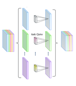
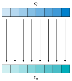
2.2.7 Depthwise Convolution Layer
Xception: Deep Learning with Depthwise Separable Convolutions 논문(2016)
MobileNet과 같이 주로 mobile device를 위해 설계된 CNN에서 사용되는 depthwise convolution은, 하나의 입력 채널마다 별도의 필터를 적용하는 방법이다.
- $g=c_i=c_o$ 인, grouped convolution의 특수한 경우로 볼 수 있다.
 |
 |
tensor shape은 다음과 같다.
| Tensors | Depthwise Convolution |
|---|---|
| Input Features $X$ | $(n, c_i, h_i, w_i)$ |
| Output Features $Y$ | $(n, c_i, h_o, w_o)$ |
| Weights $W$ | $(c, k_h, k_w)$ |
| Bias $b$ | $(c_o, )$ |
출력 텐서의 height $h_o$ 는 다음과 같이 계산할 수 있다. ( $p$ : padding size, $s$ : stride )
$$ h_o = \frac{h_i + 2p - k_h}{s} + 1 $$
2.2.8 Dilated Convolution Layer
(생략)
2.2.9 Transposed Convolution Layer
| no stride | stride = 2 |
|---|---|
 |
 |
(생략)
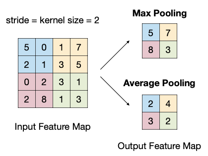
2.3 Pooling Layer
downsampling의 다른 대표적인 방법으로 pooling로, 별도의 파라미터(가중치)를 사용하지 않는다.
채널마다 적용되는 channel independent한 연산으로, 대체로 stride를 kernel size와 동일하게 설정한다.
다음은 대표적인 두 가지 pooling 방법을 비교한 그림이다.
2.4 Normalization Layer
$$ \hat{x_{i} } = \frac{1}{\sigma} (x_i - {\mu}_{i}) $$
$\mu$ : mean, $\sigma$ : standard deviation
(생략)
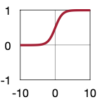
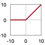
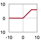
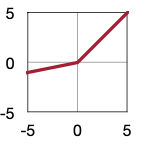
2.5 Activation Function
| Sigmoid | ReLU | ReLU6 | Leaky ReLU | Swish |
|---|---|---|---|---|
 |
 |
 |
 |
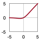 |
| $y = 1/(1+e^{-x})$ | $y = \max(0, x)$ | $y = \min(\max(0, x), 6)$ | $y = \max(\alpha x, x)$ | $y = x \cdot \sigma(x)$ |
(생략)
2.6 Transformer
다음은 transformer 아키텍처 및 Multi-Head Attention 블록의 구조를 나타낸 도식이다. Query, Key, Value의 세 가지 텐서에 attention 연산을 수행하여 출력 텐서를 산출한다.
QKV example(YouTube Search):
Q: 검색 창의 텍스트 프롬프트,K: 동영상의 제목 및 설명,V: 실제 동영상
| Transformer | Multi-Head Attention |
|---|---|
 |
 |
이때 attention 연산은 별도의 가중치를 필요로 하지 않는다.
$$ \mathbf{Attention}(Q, K, V) = \text{softmax}(\frac{QK^T}{\sqrt{d_k}})V $$
대체로 다양한 임베딩 차원 $d$ ( $d_{model}$ )에 안정적이기 위한 정규화를 수행하며, softmax를 거치면서 $N \times N$ 크기의 attention map을 획득할 수 있다. ( $N$ : sequence length )

이처럼 $N \times N$ 계산 비용을 갖는 attention map은 메모리 병목 요인에 해당한다. (토큰 수 $N$ 이 증가할수록 quadratic하게 메모리 사용량이 증가)