2 Text Classification

CMU Advanced NLP 2022 (2): Text Classification

2.1 General Framework for NLP Systems

대표적인 NLP task를 입출력 기준으로 분류하면 다음과 같다.

입력 $X$	출력 $Y$	Task
Text	Text in Other Language	Translation
Text	Response	Dialog
Text	Label	Text Classification
Text	Linguistic Structure	Language Analysis

2.1.1 Generative, Discriminative Modeling

Google Developers: What is a Generative Model?

Generative, Discriminative modeling을 통해 Text Classification을 수행하는 방법을 알아볼 것이다. 먼저 Generative Model과 Discriminative Model의 차이를 알아보자.

Generative Model	Discriminative Model

입력 샘플 $X$ 를 생성한다.	입력 $X$ 가 label $Y$ 일 확률을 반환한다.
stand alone: $P (X)$ joint(label 존재): $P (X, Y)$	conditional: $P (Y ‖ X)$

이를 text classification에 적용하면 다음과 같다.

Generative Text Classifciation

\hat{y} = a r g max_{\tilde{y}} P (X, \tilde{y})

Discriminative Text Classification

\hat{y} = a r g max_{\tilde{y}} P (\tilde{y}, X)

2.2 Generative Text Classification

먼저 다음 단어의 확률을 계산하는 language modeling은, 다음과 같이 나타낼 수 있다.

modeling 목표는 sentence, document, book 등, 어떠한 길이를 갖는 대상이든 다양할 수 있다.

P (X) = \prod_{i = 1}^{I} P (\underset{n e x t w o r d}{x_{i}} | \underset{c o n t e x t}{x_{1}, \dots, x_{i - 1}})

관건은, 어떻게 $P (X)$ 를 계산할 것인가이다.

2.2.1 Simplest Language Model: Count-based Unigram Models

먼저 다음과 같은 가정을 통해, 매우 간단한 language model을 설계할 수 있다.

Independence assumption

다음 단어의 확률은, 이전 단어들의 확률과 무관하다고 가정한다.

P (x_{i} | x_{1}, \dots, x_{i - 1}) \approx P (x_{i})

count-based maximum-likelihood estimation

다음 단어의 확률은, 특정 단어가 나오는 빈도수(count)를 센 뒤, corpus의 전체 단어 수로 나누어 계산한다.

P_{M L E} (x_{i}) = \frac{c_{t r a i n} (x_{i})}{\sum_{\tilde{x}} c_{t r a i n} (\tilde{x})}

하지만 간단한 만큼 가지고 있는 문제점도 많다.

(-) 학습 데이터에 없는 unknown word(unk)는, 확률로 0을 갖게 된다.
(-) 모든 단어에 대해, distribution을 계산해야 한다.
character/subword-based model

spelling에 기반하여 단어의 확률을 계산한다.
uniform distribution

충분한, '고정'된 크기를 갖는 vocabulary( $N_{v o c a b}$ )를 기반으로, 모든 단어의 확률을 계산한다.

참고로 unknown word 문제는, $λ_{u n k}$ 계수를 추가하여, 두 가지 확률로 구성된 식으로 구성하여 보완할 수 있다.

P (x_{i}) = (1 - λ_{u n k}) * P_{M L E} (x_{i}) + λ_{u n k} * P_{u n k} (x_{i})

2.2.2 Parameterizing in Log Space

확률의 곱은, 로그 확률의 덧셈으로 표현할 수 있다. 이러한 표현은 계산에서 안정성과 다양한 편의성을 제공한다.

P (X) = \prod_{i = 1}^{| X |} P (x_{i}) \to \log P (X) = \prod_{i = 1}^{| X |} \log P (x_{i})

특정 단어에 대한 로그 확률은 다음과 같이 표현할 것이다.

θ_{x_{i}} : = \log P (x_{i})

2.2.3 Generative Text Classifier

generative text classifier의 joint probability는, 다음과 같이 조건부 확률 기반으로 표현할 수 있다.

P (X, y) = P (X | y) P (y)

이를 통해 확률을 class-conditional language model의 관점에서 해석할 수 있고, 각 항은 다음과 같은 의미를 갖는다.

$P (X | y)$

입력이 해당 클래스와 얼마나 일치하는지를 나타낸다.

$P (y)$

class prior probability (bias)

P (y) = \frac{c (y)}{\sum_{\tilde{y}} c (\tilde{y})}

2.2.4 Bag-of-Words Generative Classifier (BoW)

다음은 Naive Bayes로 종종 지칭되는, bag-of-words generative classifier의 예시이다.

bag-of-words

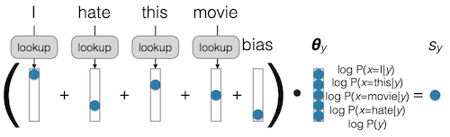
$θ_{y}$ : parameter vector

입력마다 각 클래스에 해당될 확률을 출력한다.

$S_{y}$ : score

2.3 Discriminative Text Classification

discriminative model를 사용함에 있어서, 입력을 modeling하는 데 그만큼 많은 capacity가 필요하다는 점에 유의해야 한다.

출력 확률을 direct하게 modeling하기 때문에, 뛰어난 성능을 가져야 한다.
그러나, 필요한 모든 주제를 포괄하기 위해서는, 매우 긴 학습 시간 및 자원이 필요하다.

특히, (generative model과 달리) discriminative model은 간단한 count-based decomposion으로 표현할 수 없다.

2.3.1 Discriminative Model Training

이러한 문제점 때문에, parameters $θ$ 에 기반하여, 확률을 직접적으로 계산하는 방식으로, discriminative model을 정의한다.

P (y | X; θ)

training loss function

모델 성능이 좋을수록 작은 값을 가져야 하기 때문에, negative log-likelihood를 사용한다.

ℒ_{t r a i n} (θ) = - \sum_{< X, y > \in D_{t r a i n}} \log P (y | X; θ)

optimization

\hat{θ} = a r g min_{\hat{θ}} ℒ_{t r a i n} (\tilde{θ})

2.3.2 BOW Discriminative Model

먼저, positive/negative의 간단한 이진 분류(binary classification) 문제에서, BOW discriminative model을 설계해보자.

score

s_{y | X} = θ_{y} + \sum_{i = 1}^{| X |} θ_{y | x_{i}}

score to probability (e.g. using sigmoid)

P (y | X; θ) = s i g m o i d (s_{y | X} = \frac{1}{1 + e^{- s_{y | X}}})

multi-class decision에서는, softmax를 사용하여 확률을 계산한다.

P (y | X; θ) = \frac{e^{s_{y} | X}}{\sum_{\tilde{y}} e^{s_{\tilde{y} | X}}}

2.4 Evaluation

generative, discriminative model을 모두 설계했을 때, 어떤 것이 더 좋은 모델인지를 판단할 방법이 필요하다.

2.4.1 Accuracy

가장 간단한 평가 방법으로는 accuracy가 있다.

문제는, task에 따라서 accuracy가 기만적으로 작용할 수 있다는 점이다. 만약, 여러 게시글을 입력으로, 스팸 분류기나 욕설 분류기에서 99% 정확도를 얻었다고 하더라도, 실제로 게시글에 포함된 스팸이나 욕설 자체가 1%에 불과하다면, 이는 쓸모가 없는 분류기가 될 것이다.

a c c (𝒴, \hat{𝒴}) = \frac{1}{𝒴} \sum_{i = 1}^{| 𝒴 |} δ (y_{i} = {\hat{y}}_{i})

2.4.2 Precision/Recall/F1

특정 class(대체로 minority)에 관심을 갖는다면, precision, recall, F1 등의 평가 방법을 사용할 수 있다.

관심 있는 클래스를 "1"로 지칭한다. (스팸 메세지, 욕설 등)

Precision

모델이 "1"로 분류한 출력에서, 실제 "1"에 해당되는 비율

e.g. 스팸 메세지로 분류한 출력에서, 실제 스펨 메세지의 비율

p r e c (𝒴, \hat{𝒴}) = \frac{c (y = 1, \hat{y} = 1)}{c (\hat{y} = 1)}

Recall

실제 "1"인 데이터 중, 모델이 "1"로 분류한 비율

e.g. 실제 스펨 메세지 중, 스팸 메세지로 분류한 비율

r e c (𝒴, \hat{𝒴}) = \frac{c (y = 1, \hat{y} = 1)}{c (y = 1)}

F1 Score, F-measure

precision과 recall의 조화 평균

F_{1} = \frac{2 \cdot p r e c \cdot r e c}{p r e c + r e c}

2.4.3 Statistical Testing

The Hitchhiker’s Guide to Testing Statistical Significance in Natural Language Processing 논문(2018)

예를 들어, 다음과 같이 두 모델이 비슷한 정확도를 가지고 있다고 하자.

	Dataset 1	Dataset 2	Dataset 3
Generative	0.854	0.915	0.567
Discriminative	0.853	0.902	0.570

이러한 차이가 단순히 데이터셋에 따른 차이인지, 일관적인 추세인지 확인하기 위해서는, statistical testing(significance)이 필요하다.

2.4.3.1 Statistical Testing: Basic Idea

p-value
confidence interval

(생략)

2.4.3.2 Unpaired vs. Paired Tests

	Unpaired Test	Paired Test

(생략)

2.4.3.3 Bootstrap Tests

(생략)